

In this blog, I publish an article I wrote to take part in “SIAT Technical Analyst of the Year 2021” competition. Due to the length and quantity of the topics covered, I thought useful to split it into four parts. In the second one, we will deal with the synthetic time series and their importance to create a predictive model of the maximum Drawdown.
Creating Synthetic Time Series
One of the main bottlenecks that analysts run into, is the challenge of having enough data. If we need time series to test our strategies, or if we need more data to train Machine Learning algorithms so as to build better models, the use of synthetic data may be the answer.
As the word suggests, synthetic data are artificially made, with the constraint of maintaining the same features of the data collected in the real world. The use of synthetic data is incredibly growing, companies like Amazon have turned their attention to synthetic data to generate the large amount of datasets required to train Alexa in new languages(1), or Google has started a project to create synthetic medical images to generate models that help doctors’ diagnosis(2).
Using a statistical approach for the study of the DrawDown, it inevitably requires historical series that are large enough over time and above all that are in large quantity to cover each case.
The twelve real time series previously chosen are not enough for an accurate statistical analysis and especially to train a Machine Learning algorithm, therefore the opportunity to use synthetic time series is affordable and nowadays it is inexpensive too, unlike a few years ago when sophisticated software and people who knew how to use them were required. Using synthetic time series is an opportunity that we do not miss.
The method we are going to implement to make the time series, is essentially build on the Wiener process. It is usually used to create a Brownian motion and it has the capability to return an equity line that has statistical features, as mean and standard deviation, set as from the start. Its general formulation is as follows:
Yi = Yi-1 ∙ ( 1 + μ * ( ti – ti-1 ) + σ * radq( ti – ti-1 ) * Xi )
Where:
- ti is the i-th time instant;
- Yi is the value of the equity line at ti time;
- Xi is a random independent variable with standard normal distribution;
- μ and σ are the parameters used by Wiener process;
In our case, we take the following assumptions:
- The synthetic time series will have a daily timeframe, while the time intervals ti-ti-1 are always constant and equal to 1;
- μ and σ are the expected mean return and standard deviation, respectively.
The formula takes the following expression:
Yi = Yi-1 + Yi-1 ∙ ( μ + σ Xi )
Where the term inside the brackets is the percentage return on day i:
ri = μ + σ Xi
If we chose to use logarithmic returns, we can take advantage of the properties of logarithms and find average, partial and total returns with simple sums. Therefore, if we define the return as logarithmic, we will find that the is the cumulative logarithmic return on the i-th day:
Ri = ln( Yi / Y0 ) = ∑(k=1,i) rk = ∑(k=1,i) ( μ + σXk )
The value of the Equity Yi becomes:
Yi = Y0 * e∑(k=1,i)(μ+σXk)
An example can help us to understand how this formula works. Set σ=10%, μ=5% and Y0=100€, we find:
| ti | Xi | ri = μ + σXi | Ri = ∑(k=1,i)rk | Yi = Y0 ∙ eRi |
|---|---|---|---|---|
| 1 | 0.5 | 12.5% | 12.5% | 113€ |
| 2 | -0.2 | 9.0% | 21.5% | 124€ |
| 3 | 0.1 | 10.5% | 32.0% | 138€ |
| 4 | 0.0 | 10.0% | 42.0% | 152€ |
Where Xi re the random numbers with a standard normal distribution and Yi is the synthetic equity line.
The model shown was implemented as follows:
- First, we set the quantity of time series that will make up the dataset and the number of epochs for each sample. On this occasion, we take 2048 time series and 20°000 epochs – big numbers but they guarantee a good training and a fine statistical accuracy.
- Next, we establish the ranges for the mean and standard deviation of the returns. To compare this synthetic dataset with the real one, we chose two range that contain the real time series listed in table 2:
- μ = ( 0.005% – 0.035% )
- σ = ( 0.05% – 1.50% )
- To explore the potential relationship between the MDD and the time period, we decide to also change the length of the epochs of each series, inside a range of 8 -32 values.
- For each of the 2048 synthetic time series, the code randomly set the mean, the standard deviation and the period within the range provided, then it will calculate 20°000 equity lines and the related 90MDDs.
- The results found are saved and stored in a database, which we will call synthetic data dataset.
In allegato è disponibile il codice, sia per consultazione sia per chi volesse testarlo in proprio, mentre nella tabella 4 si riporta un estratto dei risultati presenti nel dataset.
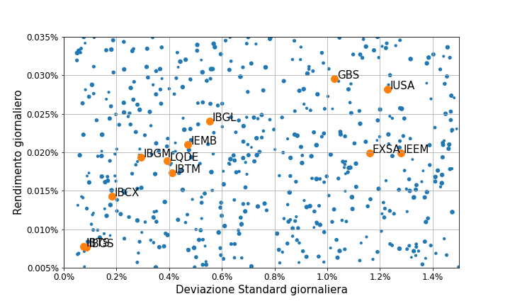
The chosen parameters immediately suggest that the amount of synthetic data is not comparable at all with the real ones. Having 2048 time series with very different features is something that is difficult to find in world financial markets. Figure 6 shows the positions of 512 synthetic time series (a quarter of the entire dataset) within the risk – return diagram and, for comparison, there are also the positions of the twelve real time series. The spread on the chart is wide, covering an almost complete spectrum of all combinations of risk and return.
| Time Series | Mean Return | St.Dev. Return | Period of epoch | 90MDD |
|---|---|---|---|---|
| 1 | 0,0307% | 1,39% | 15 | 8,10% |
| 2 | 0,0097% | 0,37% | 20 | 2,60% |
| 3 | 0,0325% | 0,48% | 31 | 3,94% |
| 4 | 0,0052% | 1,47% | 13 | 8,13% |
| … | … | … | … | |
| 2048 | 0,0164% | 0,90% | 10 | 4,22% |
Having 20°000 epochs with an average period of 20 values brings to get 400°000 values, equal to 16 centuries! It may seem like an excess but it allows to find excellent accuracy. The comparison between figure 3 and figure 7 is explanatory of this advantage, the very high number of epochs allows to get an excellent approximation of the probability distribution of the cumulative returns Ri and of the MDD, respectively to the Gaussian and to the log-normal (orange lines), difficult to achieve with real time series.
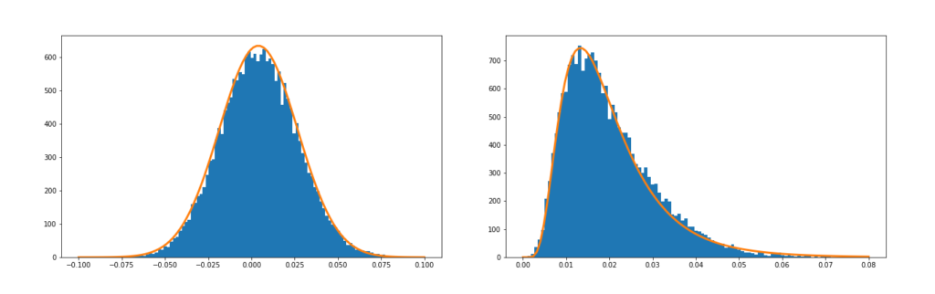
for a generic synthetic time series
The synthetic time series solve the weakness of the real series in a single shot, a few lines of code can generate very high numbers of information. There may be doubt about this kind of time series that is born in the laboratory, but these products are not the goal but the boost to train a Machine Learning algorithm.
1) https://www.amazon.science/blog/tools-for-generating-synthetic-data-helped-bootstrap-alexas-new-language-releases
(2) https://ai.googleblog.com/2020/02/generating-diverse-synthetic-medical.html
Annex
Here below there is an extract of the code used to carry out the numerical analyzes.
Importing Libraries:
from scipy.stats import norm
import numpy as np
import pandas as pd
import sqlite3 as sql
defining the number of samples and epochs, making the DataFrame used to record the results:
samples = range(1, 2048 + 1)
epoch = range(1, 20000 + 1)
DATASET = pd.DataFrame(index = samples, columns = ['media', 'devst', 'periodo'])
TARGET  = pd.DataFrame(index = samples, columns = ['MDD'])
Nested loop, in the outer one the value of mean, standard deviation and period of the epoch are randomly defined within fixed intervals, in the inner one the equity and the 90th percentile of the MDD are calculated:
for j in samples :
    Risultato = np.zeros( ( len(epoch) ) )
    media     = np.random.uniform(low = 0.00005, high = 0.00035)
    devst     = np.random.uniform(low = 0.0005, high = 0.0150)
    periodo   = np.random.randint(8, high = 32, size = None, dtype = int)
    for i in epoch :
        LogReturn = norm.rvs(loc = media, scale = devst, size = periodo)
        cumulato = np.cumsum(LogReturn)
        Equity = 1000 * np.exp(cumulato)
        DD_rif = np.maximum.accumulate(Equity)
        DrawDown = (DD_rif - Equity) / DD_rif
        Risultato[i-1] = DrawDown.max()

    DATASET.loc[j, 'media'] = media
    DATASET.loc[j, 'devst'] = devst
    DATASET.loc[j, 'periodo'] = periodo
    TARGET.loc[j, 'MDD'] = np.percentile(Risultato, 90)
Saving the results in a database:
conn = sql.connect('Synthetic.sqlite')
cur = conn.cursor()
cur.execute( 'CREATE TABLE IF NOT EXISTS dataset (
    "indice" INTEGER NOT NULL UNIQUE,
    "media" REAL,
    "devst" REAL,
    "periodo" REAL,
    "MDD" REAL,
    PRIMARY KEY ("indice" AUTOINCREMENT) );' )

for i in range(DATASET.shape[0]) :
    cur.execute( 'INSERT INTO dataset
        (media, devst, periodo, MDD) VALUES (?, ?, ?, ?)',
        (DATASET.iloc[i, 0],
         DATASET.iloc[i, 1],
         int(DATASET.iloc[i, 2]),
         TARGET.iloc[i, 0]) )
    conn.commit()
cur.close()
If you have any questions to ask me, do not hesitate to write to me in the form below, otherwise you can find me on Facebook and LinkedIn. If you want to stay up-to-date and not miss any article as soon as it comes out, subscribe to the newsletter by filling out the following form:
If you like my articles and MP Investit project, you can support me with a free donation with PayPal or with a Brave browser reward. This encourage me to produce better and better content. Thank you!