

In this blog, I publish an article I wrote to take part in “SIAT Technical Analyst of the Year 2021” competition. Due to the length and quantity of the topics covered, I thought useful to split it into four parts. In this third part, we are going to see how to train the algorithm and to validate our predictive model of the maximum drawdown.
Changing Point of View with Machine Learning
In a typical situation of algorithmic trading, the trader that is going to create a Trading System, codes in a programming language the rules of his/her strategy in an extremely precise way, such as: buy and sell, filters, risk management, parameters and constraints. When the Trading System is implemented and launched in “live”, it get the flow of data arriving from the market, it processes them according to the rules written by his/her programmer and then it returns the buy and sell signals.

With Artificial Intelligence and especially with Machine Learning, the paradigm is turned. An effective definition of Machine Learning is the following:
“Machine learning is the science (and art) of programming computers so they can learn from data”
from Aurélien Géron’s book “Hands-on Machine Learning with Scikit-Learn and TensorFlow”
The rules of the game are no longer defined by human but it is the machine that learns by itself what are the best rules that fit the data input into the answers. The new paradigm is divided into two distinct phases:
- in a first part, called the training phase, the so called “Machine Learning Algorithm” takes both the data input and the answers, then it creates a model that contains the rules that link inputs and outputs;
- in the second part, called the inference phase, the model is fed by the data input and according with its rules, it makes its prediction.

In the same way as the trader – programmer, who “trains” him/herself through the time series to find the rules of his/her Trading System, the machine “trains” itself with the data to designs its model. But, between the two paradigms, which is better? The human mind is unmatchable, an innovative idea can always make the difference in solving a problem, but when it’s time to come up with numbers to pull out other numbers, the machine doesn’t lose a challenge and it does its work at an incredible speed. At the end, which of them do we choose? It depends on how much data are available. If we have a lot of data, such as numerous and deep time series, a Machine Learning algorithm is able to explore the whole set and especially with no bias. On the other hand, if the financial market where we operate has little information or it is difficult to access, or more simply there are no long time series, the intuition of the trader – programmer is essential in defining the Trading System.
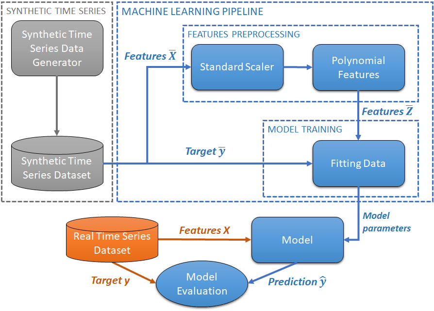
Coming back to our prediction of the MDD, synthetic time series allow us to move the balance of a situation towards the field of activity of Machine Learning. In figure 10 we can see what the sequence of events is: after generating the synthetic time series dataset, the data is pre-processed and subsequently used to train the Machine Learning algorithm, which will produce the model; for the final evaluation, the model predictions are compared with the real time series data dataset.
In the following paragraphs we are going to see in detail how the blue modules, shown in figure 10, work.
Standardize and Normalize
Our dataset (see table 4) consists of the two features, “mean” and “standard deviation”, with very low nominal values, even lower than one thousandth, and one feature, “epochs”, with values greater than unity.
It is usually to have features with different orders of magnitude. These large differences in scale are not optimal for learning algorithms, because they would not be able to put all features on the same level of importance, with the risk that one feature overlooks the others reducing the learning capabilities, as well as potential issues on the stability of the computational methods. The solution for this occurrence is the scaling techniques, which modify the range of the features to bring them to the same size.
The SciKit-Learn library provides the StandardScaler function, which is widely used to “standardize” the scale of features during the data preprocessing. The StandardScaler function returns new features that have “standard” distributions, with a mean equal to zero and a normalized distributions, meaning a standard deviation equal to one, produced by the original ones by applying the formula:
zi = ( xi – X ) / Sx
the result is new Z features that have the same size and stand on the same range of values.
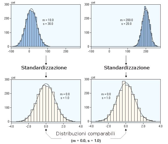
(1) Figure taken from website https://www.lorenzogovoni.com/ridimensionamento-dei-dati/
Multiple Linear Regression
Among the machine learning algorithms examined, Multiple Linear Regression (MLR) is the choice because it provides a good tradeoff between accuracy and simplicity, as we will see soon. This algorithm is suitable when the dependent variable has a potential linear relationship with its independent variables. The general form is shown below:
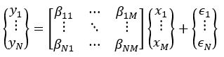
where:
- yi is the value of the i-th component of the dependent variable,
- βij is the coefficient of the linear regression,
- xj is the value of the j-th component of the independent variable,
- εi is the residual value which depends on non-linear terms
The algorithm used is the LinearRegression of the SciKit Learn library, which has a formula that links the target value and the independent variables in a linear combination:
ŷ(β, x) = β0 + β1x1 + ··· + βMxM
Where ŷ = y – ε is the value predicted by the model. The values of the coefficients used by the model are obtained from the sample values xj(k) and y(k) Where is the value predicted by the model. The values of the coefficients used by the model are obtained from the sample values e from the dataset, finding the minimum of the following cost function:
min||Xβ -y||22
in other words, the model uses the samples coming from the dataset and it finds the coefficients βi which minimize the sum of the squares of the residuals ε(k).
The LinearRegression algorithm manages only one value ŷi, if the dependent variable has two or more values it is necessary to create and train more models. In our case we have only one target, 90MDD, therefore it is enough to train a single LinearRegression algorithm.
Polynomial Regression
In Machine Learning projects, a common practice is to take linear regression models and fit them on datasets that are governed by nonlinear functions. This approach allows to maintain the low computational costs typical of linear models, but to be used to a wide number of scenarios.
The most used method is to take a linear regression and to create new polynomial independent features. For example, we might have a linear model with only two variables like this:
ŷ(β, x) = β0 + β1x1 + β2x2
If our data samples follows a parabolic function, the variables x1 and x2 can be combined to create new second degree terms:
ŷ(β, x) = β0 + β1x1 + β2x2 + β3 x1x2 + β4x12 + β5x22
Although it doesn’t seem like it, this new model can always be handled as a linear model, if we replace the x variables with a new set of z variables, then it becomes clearer:
ŷ(β, z) = β0 + β1z1 + β2z2 + β3 z3 + β4z4 + β5z5
We can see how the new model remains linear and so linear regression training methods can be used. A creation of a larger space provides a model with a better flexibility and the capability to get to a large amount of datasets.
The SciKit Learn library is able to train a polynomial regression algorithm, taking care of transforming the features, leaving to the programmer only the choice of the degree term of the new terms.
Once the data collection and preparation phase and the choice of the Machine Learning algorithm have been completed, in the fourth and last part of this article finally we are going to create the predictive model and to analyze its results.
If you have any questions to ask me, do not hesitate to write to me in the form below, otherwise you can find me on Facebook and LinkedIn. If you want to stay up-to-date and not miss any article as soon as it comes out, subscribe to the newsletter by filling out the following form:
If you like my articles and MP Investit project, you can support me with a free donation with PayPal or with a Brave browser reward. This encourage me to produce better and better content. Thank you!