

In this blog, I publish an article I wrote to take part in “SIAT Technical Analyst of the Year 2021” competition. Due to the length and quantity of the topics covered, I thought useful to split it into four parts. In the first one, we will see how to measure risk by means of Drawdown.
Abstract
In last decades, we have seen an increasingly use of statistical and IT methods for the Technical Analysis of the financial markets, real drivers in the growth of study and decision-making skills both of traders and investors. The factors that played a major role in this revolution were the availability of many and large time series, good computing power and Technical Analysis software platforms. Unfortunately there were some cons, in order to be up to date it was necessary to have proprietary software and adequate IT infrastructures, which required economic and time resources for learning to use them.
Today, this information revolution is experiencing a new boost, making new technologies more accessible. Fitting performance of Personal Computer, the availability of high-level programming languages, free access to data, in addition to open source policy that reduces costs – these allow a wide audience of technical analysts to manage complex analysis scenarios on their own.
The following article has the target to set a low-cost analysis that uses the latest Information Technologies, by computational simulations and machine learning models. As a case study, we will perform an analysis of maximum drawdown and we will propose a model to predict it. The framework of the article is as follow:
- In the first part, we are going to take a group of twelve time series that are representative of the main financial assets, we will analyze their probability distribution function for Maximum DrawDown, then we will infer the results to a more general cases.
- In the second part, we are going to see how to build a group of synthetic time series, these will have both size and statistical accuracy large enough to fulfill Machine Learning training needs.
- In the third part, we are going to introduce a Machine Learning algorithm, that will be trained to create a model to predict the Maximum DrawDown of a generic time series.
- In the fourth part, the performance of the model will be evaluated through a direct comparison with the time series shown in the first part.
The analyses, and all the computation, are achieved with the Python programming language and with its libraries Numpy, Pandas, Matplotlib, Sci-Kit Learn and SQLite. This combination of software is the most powerful and most used in the world of Data Science, it’s accessible to everyone thanks to free distribution, with no cost and with a plenty of free on-line courses to learn how to use it.
Measure the Risk with the Drawdown
The Maximum DrawDown (MDD) of a time series is defined as the maximum difference from a relative maximum to a following relative minimum, that can be found in a specific time range. In the field of Trading and Investing strategies, the MDD is a measure of risk and it is frequently used to evaluate the performance of portfolios and Trading Systems. The relevance of the MDD lies that it represent the maximum loss that a trader / investor can incur if he / she goes to market and the he / she exits at the worst time (go when prices are high, exit when prices are low).

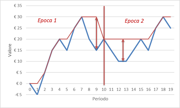
The MDD can be computed in the following way, starting from values Yu from time series (blue line, figure 1). The relative maximum of the time t (red line) is defined as:
St = max( Yu , u ≤ t )
Then, for each point of the time series, the DrawDown is computed as the difference between the relative maximum and the time series:
DD_t = St – Yt
While the MDD of a period [ 0, T ] is:
max u ∈ [ 0, T ] ( DDu )
The MDD depends on a long list of factors, the main ones are:
- The average return;
- The standard deviation
- The sampling frequency;
- The sequence of the all values of the series;
- The width time range
All these factors contribute to the avaluation of the MDD and they cannot be disregarded when comparing two or more strategies with the same MDD.
The MDD is very popular as a measure of risk in the financial field, its explanation is very intuitive compared to others, but unfortunately the MDD has a lack of an effective analytical method to find the solution starting from a generic time series, leaving the issue to computational analysis, furthermore it has an high sensitivity to the initial conditions that leads to a large measurement error.
Time series, that we are going to use, are chosen with the following criteria:
- Great depth of data, to take the main market phases of the last years. As basic rule, it is required to begin no later than 2007;
- Total return series, to have a large homogeneity an to avoid gaps due to distribution of dividends or coupon;
- Wide diversification, to cover all the main assets and to have the greatest geographical and capitalization coverage.
Table 1 showns the selected stocks, with the most important information. The almost exclusive presence of iShares products in not a coincidence, because of the US firm provides for free data of its ETFs and with the greatest depth available on Borsa Italiana, in some cases they starts from 2003-2004, with the benefit to cover important and critical market phases, as the 2008-2009 US subprime mortgage crisis, the 2011-2012 Euro crisis and the actual 2020-2021 Covid-19 pandemic.
| Ticker | Asset | Category | Starting from | N. Available value |
|---|---|---|---|---|
| IBGS.MI | Liquidity | Euro Government Bond 1-3yr | 05.06.2006 | 3823 |
| IBTS.MI | Liquidity | Treasury Bond 1-3yr | 05.06.2006 | 3819 |
| IBGM.MI | Bond | Euro Government Bond 7-10yr | 08.12.2006 | 3691 |
| IBGL.MI | Bond | Euro Government Bond 15-30yr | 08.12.2006 | 3687 |
| IBCX.MI | Bond | Euro Corporate Bond | 17.03.2003 | 4647 |
| IBTM.MI | Bond | Treasury Bond 7-10yr | 08.12.2006 | 3683 |
| LQDE.MI | Bond | USD Corporate Bond | 16.05.2003 | 4588 |
| IEMB.MI | Bond | USD Emerging Markets Bond | 15.02.2008 | 3386 |
| EXSA.MI | Stocks | Stoxx Europe 600 | 13.02.2004 | 4369 |
| IUSA.MI | Stocks | S&P 500 | 15.03.2002 | 4883 |
| IEEM.MI | Stocks | MSCI Emerging Market | 18.11.2005 | 3970 |
| GBS.MI | Commodities | Physical Gold | 29.03.2004 | 4386 |
Using the times series from ETFs, rather than to go straight with indices, it is justify for guarantee a target of this article, to maintain an high level of affordability for analysis. ETFs / ETCs companies provide historical NAV for free and these are easily available on their websites, furthermore the NAV is an official value declared to Borsa Italiana, a cheaper and more accessible solution for everyone than buying historical time series from financial service provider. Unfortunately there is also disadvantages, the NAV has only daily values without intraday information, restricting the analysis over long timeframes.
Time series shown in table 1 were downloaded in Excel format at the end of April 2021 frow internet and loaded into a database in SQLite format, a public domain library already embedded in Python.
In order to have a suitable amount of data to work on, the MDD will be not calculated over the whole time range available, but each of the twelve time series will be split into many little intervals of equal length, so a large quantity of MDDs are available. For this article, we have chosen a range of 20 values, that brings to about one working calendar. Figure 2 clarifies what it means: for instance, if we divide a time series with 20 values into two ranges, we own two MDDs (vertical lines with double arrows). Each range will take the name of Epoch, from our historical time series we have a minimum of 169 to a maximum of 244 epochs for each series, with the same number of MDDs.
With the aid of Python programming, it is possible to calculate with an extreme speed all the epochs and the related MDDs of the historical time series, later to visualize with histograms the probability distributions of the MDDs (figure 3). The obtained graphs show how the MDDs concentrate around a very narrow range and how they tend towards the right side drawing a long tail, these can be explained as the epochs have a MDDs basically constant, even if many times a wide MDD is present, a coherent behavior with the nature of MDDs and with the risk to incur in large losses when events are adverse.
From a statistical point of view, we cannot shape MDD probability distributions to a Gaussian one, therefore it is not possible to use, as usual, the mean and the standard deviation to define their characteristics. Academic studies have demonstrate that if ideal time series, such as those created by Brownian motion, then MDD probability distributions are similar to log-normal ones, a type of asymmetric distribution that is often come with random variables that only assume positive values, as exactly the MDD.
Figure 4 shows an example of an ideal log-normal probability distribution for MDD. Among all these values, we are going to assume the 90 percentile as the MDD of our interest, meaning this value enclose 90% of the observed MDD on its left side and we call it with the abbreviation 90MDD. Explanation for percentile is not so far from Value at Risk (VaR), that tries to estimate the maximum potential loss at a fixed level of confidence and time horizon.

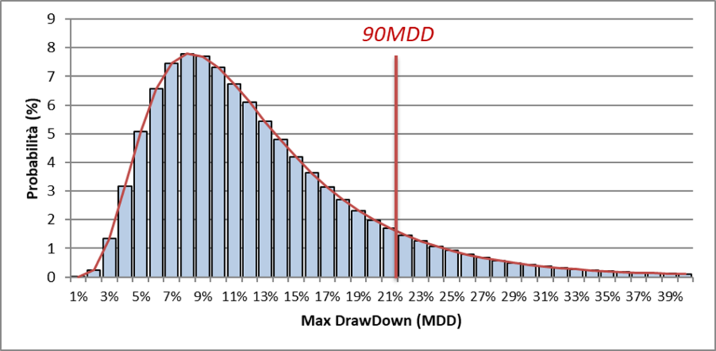
Using a single value as representative sample of the whole MDD probability distribution, it allows a more direct comparison between various analysis results. We recall that 90MDD is an arbitrary value, we could take any other point of the distribution, such as the mode (the value with the high frequency) or the arithmetic mean or the median.
Python can calculate the percentile from any distribution and it can create a table that shows, for every time series, the average and the standard deviation of daily logarithmic returns, the 90 percentile of the MDD on epochs with 20 values-long.
| Time Series | Average of Returns | St.Dev. of Returns | 90MDD |
|---|---|---|---|
| IBGS | 0,008% | 0,08% | 0,5% |
| IBGM | 0,019% | 0,29% | 1,9% |
| IBGL | 0,024% | 0,55% | 4,0% |
| IBCX | 0,014% | 0,18% | 1,3% |
| EXSA | 0,020% | 1,16% | 8,1% |
| IBTS | 0,008% | 0,08% | 0,4% |
| IBTM | 0,017% | 0,41% | 2,7% |
| LQDE | 0,019% | 0,39% | 2,5% |
| IUSA | 0,028% | 1,23% | 7,6% |
| IEMB | 0,021% | 0,47% | 3,0% |
| IEEM | 0,020% | 1,28% | 9,2% |
| GBS | 0,030% | 1,03% | 7,3% |
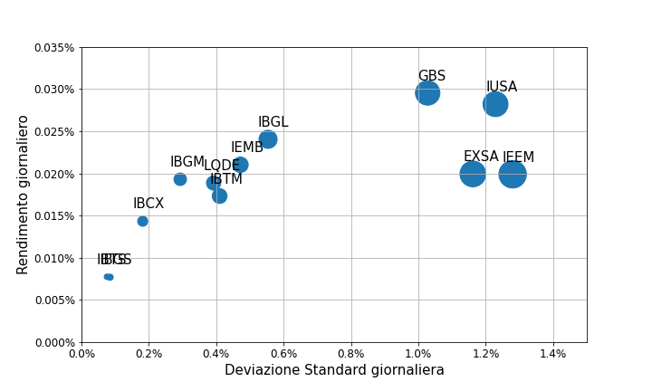
Table 2 shows data that we indicate as Real Time Series Dataset, it will be used in the next chapters to test the capabilities of the Machine Learning model to predict. Figure 4 visualizes the table 2, in which the circles are larger, the 90MDD is higher. It’s to be noted that the value of 90MDD is proportional to the standard deviation, a perfect indication that some relationships between the two features exists and that we can explored with Machine Learning algorithms.
A Machine Learning algorithm needs a large quantity of samples in order to create a reliable predictive model. Although the Real Time Series Dataset is representative of financial markets and years wide, twelve samples generated over a few hundred epochs are not enough for our purpose. To resolve the issue, we can add assets more, but in the next section we will see a better and more effective method.
If you have any questions to ask me, do not hesitate to write to me in the form below, otherwise you can find me on Facebook and LinkedIn. If you want to stay up-to-date and not miss any article as soon as it comes out, subscribe to the newsletter by filling out the following form:
If you like my articles and MP Investit project, you can support me with a free donation with PayPal or with a Brave browser reward. This encourage me to produce better and better content. Thank you!