

(Cover image: created by Bing Image Creator using DALL·E 3 technology)
Let’s imagine our investment portfolio as a soccer team. Each portfolio component plays a distinct role, akin to players fulfilling specific tasks like defenders, midfielders, forwards, and so on. In a successful soccer team, it’s crucial for each player to best in their role, leveraging their unique skills, and for the team to strike a balance between offense and defence.
We’d never dream of putting a striker in goal or building a team made entirely of defenders! Instead of focusing solely on offense – such as chasing returns from a single asset class – the coach works to balance the game between attack, midfield, and defence. This means balancing return and risk across various asset classes. This way, even if the defensive line (one asset class) doesn’t score many goals, it significantly contributes by preventing them (preserving capital and minimizing losses), which is essential to winning the game.
Furthermore, within the three main sections of the team, assigning the right roles to individual players is critical. Some players are better suited for the wings, while others excel in central positions – just as in each asset class, certain instruments and products are better equipped to fulfill specific functions.
Just as an experienced soccer coach balances the team to achieve the optimal mix of offense and defense, we introduce a new coach for our portfolio: the Hierarchical Equal Risk Contribution (HERC) algorithm. This algorithm can optimize the selection of financial instruments (our roster of players) to ensure stable and sustainable long-term performance, helping us reach our financial goals—like a soccer team striving to win the championship.
HERC is an emerging approach that offers a unique perspective on portfolio construction. It is grounded in solid principles of diversification and risk management, helping investors achieve greater stability between expected returns and the risks associated with their investments.

Understanding HERC
The concept of HERC belongs to the family of allocation strategies built on Risk Parity. The theory behind HERC is simple yet powerful, and it can be summarized in two key steps:
- Organize a portfolio using hierarchical clustering;
- Allocate capital in a top-down cascade along the hierarchical structure.
The first step was discussed in our previous article, Machine Learning Reshapes Classification Rules, where we explored the world of hierarchical clustering. We demonstrated its remarkable ability to recognize meaningful structures and connections among financial instruments. Specifically, we saw how machine learning algorithms can group the companies comprising the FTSE MIB index, offering fresh perspectives for portfolio analysis and management by creating order without bias notions or predefined frameworks.
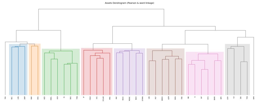
In Figure 2, we can observe the dendrogram of the FTSE MIB, featuring eight distinct colored rectangles representing groups of companies. Examples include the “Utility Group” (green rectangle), which includes Hera, ENEL, A2A, Italgas, Snam, and Terna, and the “Banking Group” (pink rectangle), which contains major Italian banks known for their strong correlations. The hierarchical clustering algorithm tops at interpreting price dynamics, providing a fascinating perspective on the hidden connections between different companies within the FTSE MIB. This process creates a structure that reflects the relationships and similarities among the companies, unveiling the links between the members of our index.
Risk Parity strategies allocate more resources to financial instruments with lower risk and less to those with higher risk, aiming for equally distributed risk contributions. HERC takes this idea one step further: balancing marginal risk contributions not only applies to individual instruments but also follows the hierarchical structure, addressing every branch of the tree.
This hierarchical risk allocation allows for greater precision in portfolio management. It accounts not only for the volatility of individual instruments and their correlations, as in the classic Risk Parity approach, but also for their interactions and relationships within the portfolio. This enables a more comprehensive and sophisticated approach to risk management.
At first glance, this concept might seem a bit complex, but let’s clarify it with a simple example using Figure 3. Imagine a portfolio with 10 instruments, labelled from A to L, and we want to distribute the available capital among them. We start by using the historical data of these instruments to create a hierarchical tree, following the clustering method described in our previous article. In Figure 3, three groups are formed, with the blue and orange groups closer to each other, while the green group stands farther apart.

Now, imagine we are at the top of the tree with the entire capital at our disposal, and we begin moving down the branches. At the first split, the capital is divided equally between the left and right branches. As shown in the figure, 50% goes to the left, where a further split divides the capital again: 25% goes to the blue group and another 25% to the orange group. Meanwhile, the 50% allocated to the right flows directly to the green group. The final step involves evenly distributing the capital among the instruments within each group. For instance, the four instruments in the blue group each receive 25% / 4 = 6.25% of the capital.
This straightforward use of hierarchical clustering is known in finance as Hierarchical Clustering Asset Allocation (HCAA). HCAA and HERC are closely related, with the primary difference being that while HCAA divides capital equally at each branch, HERC focuses on equally distributing marginal risk contributions.
The Mathematical Model
As usual in our articles, we dedicate a section to the mathematical details, allowing those who appreciate the elegance of mathematics to understand the inner workings of the HERC algorithm. Just as gears, escapements, and balances bring grace to the inner mechanisms of a wristwatch, understanding the mathematical components of HERC enables us to admire its sophisticated design. However, for those who prefer to focus on external beauty – like the watch’s dial and crown—this section can be skipped entirely, and one can still enjoy the refined functionality of HERC without delving into its inner workings.
In August 2018, Thomas Raffinot, a brilliant French quantitative economist, introduced the world to an academic paper titled The Hierarchical Equal Risk Contribution Portfolio. In his work, Raffinot unveiled an innovative algorithm that leverages advanced statistical and machine learning techniques.
Once the portfolio basket is selected, the algorithm determines the weights of each component through four key steps:
- Hierarchical clustering is applied to the portfolio basket.
- The optimal number of groups is determined.
- Capital is allocated using an iterative top-down division along the hierarchical structure.
- Risk is evenly distributed within each individual group.
1. Hierarchical Clustering
As we explored in the previous article, the hierarchical clustering algorithm proves remarkably effective in segmenting and organizing our basket of asset classes. This process relies on its ability to identify the unique characteristics of historical series and the similarities between them.

To clearly visualize the results obtained through hierarchical clustering, we can refer to Figure 4, which shows a dendrogram. This graph is ideal for representing the hierarchical structure of the connections among the elements in a portfolio, providing a clear and intuitive visual representation.
2. Optimal Number of Groups
Deciding on the number of groups to categorize the elements in a portfolio is a critical step. In many cases, this decision is arbitrary – we might choose a small number of groups to capture the primary investment categories or delve into a finer division, creating numerous groups, each with its own unique characteristics. In Figure 2, we observed how the companies comprising the FTSE MIB were grouped into eight categories. This number was selected to accurately reflect the intrinsic structure of the data, avoiding both an excessive and insufficient number of groups.
The number of groups significantly influences how HERC allocates weights. The distribution between groups and within each group can vary substantially. To address this, HERC employs a method known as the Gap Index Method to determine the optimal number of groups.
Without straying too far into technical details, the Gap Index Method evaluates how “compact” the elements within each group are and tests the stability of this cohesion when the initial portfolio is altered. The optimal number of groups is the one that ensures the highest stability.
For more details and an in-depth explanation of the Gap Index Method, I encourage you to consult the dedicated article available at this link.
3. Iterative Top-Down Division
After completing the dendrogram and determining the optimal number of groups, the next step is to calculate the weights assigned to each group. This process is divided into two key stages: Calculating the risk of each group; Assigning weights to the groups.
Refer to Figure 5, which illustrates a dendrogram split into two groups – one on the left (SX) and the other on the right (DX) relative to Node A.

For each group, the risk is estimated using the individual risks of the elements within that group. For each element k belonging to group g, the weight is calculated as follows:
\tag{1a}
w_{gk}=
\frac
{\frac{1}{risk_k}}
{\sum_{\substack{m=1}}^N \frac{1}{risk_m}}
The total risk of group g is then computed as:
\tag{1b}
risk_g =
{\sum_{\substack{m=1}}^N w_{gk} \cdot risk_k }
This formula simplifies the Risk Parity approach, where weights are assigned so that each element contributes equally to the overall risk. Now, with the risks for groups SX and DX calculated, weights are distributed using these formulas:
\tag{2a}
w_{SX}=
\frac
{\frac{1}{risk_{SX}}}
{\frac{1}{risk_{SX}}+\frac{1}{risk_{DX}}}
\tag{2b}
w_{DX}=
\frac
{\frac{1}{risk_{DX}}}
{\frac{1}{risk_{SX}}+\frac{1}{risk_{DX}}}Where riskSX and riskDX represent the risks associated with groups SX and DX, respectively. Formulas (2) are analogous to (1), ensuring that marginal risk contributions are balanced between the two groups. Simply put, the higher the risk of one group, the lower the weight assigned to it.
This risk calculation and weight assignment process is performed at every node, moving from the top of the hierarchy to the bottom, until reaching the group level identified in the prior phase.
In these formulas, we use the generic term “risk” because the HERC algorithm does not mandate a specific risk metric. Volatility – the most commonly used risk measure – can be successfully applied here, especially when return distributions approximate a normal curve. However, HERC allows flexibility to use alternative metrics, particularly those suited for quantifying downside risk, such as maximum drawdown. Advanced metrics like Conditional Value at Risk (CVaR) and Conditional Drawdown at Risk (CDaR), which rely on percentile functions, are also valid options.
Thomas Raffinot, the creator of the HERC algorithm, favors CDaR. According to his simulations, CDaR yields particularly compelling results, providing a more comprehensive perspective on tail risk management than traditional metrics like volatility.
4. Equal Risk Allocation
Once weights are assigned to each group, they are distributed among the individual elements within each group using the Risk Parity approach. The formula applied in this phase is the same as previously introduced:
\tag{3}
w_{gk}=
\frac
{\frac{1}{risk_k}}
{\sum_{\substack{m=1}}^N \frac{1}{risk_m}}
It’s important to note that, from a strictly mathematical perspective, this formula represents a simplified application of the Risk Parity approach. These simplifications are used to facilitate the derivation of a closed-form solution. A more detailed analysis of this aspect will be covered in a future article, where we will explore the mathematical foundations of this Risk Parity solution in greater depth.
Example
To better understand the HERC algorithm, particularly steps 3 and 4, which form the core of this approach, let’s examine a practical example. Using the dendrogram shown in Figure 5, we assign a risk value to each element and determine that the optimal number of groups is 3.
At the top of the dendrogram, we see 100%, representing the total capital to be allocated among the elements at the bottom of the dendrogram. The resulting distribution is depicted in Figure 6.

Starting at the top of the dendrogram, the weight is entirely concentrated at 100%. As we move down the tree, we reach Node A, which represents the first split: one branch leads to the green group (right), while the other heads toward the blue and orange groups (left).
To calculate the risk of the left and right branches, we refer to formulas (1a) and (1b). The table below shows the calculations for the left branch:
| Element k | Element Risk riskk | Weight Contribution wgk | Marginal Risk Contribution riskk*wgk |
| a | 16% | 4,2% | 0,67% |
| b | 16% | 4,2% | 0,67% |
| c | 2% | 33,3% | 0,67% |
| d | 2% | 33,3% | 0,67% |
| e | 8% | 8,3% | 0,67% |
| f | 8% | 8,3% | 0,67% |
| g | 8% | 8,3% | 0,67% |
The risk of the left branch is calculated by summing all the marginal risk contributions listed in the last column, resulting in 4.7%. It’s no surprise that all contributions are equal, as the Risk Parity approach inherently leads to a uniform distribution.
This iterative approach also applies to Node B, where the two branches split into the blue group and the orange group. Once the weights for these three groups are determined, the process does not continue further through nodes and branches within the groups. Instead, weights are assigned using formula (3).
Figure 7 illustrates the results of our example, with the risks of each element and branch shown in black, while the weights of each branch are indicated in red. It becomes clear that lower-risk elements receive the majority of the capital, as seen with the elements in the green group, while higher-risk elements are assigned minimal weights, such as elements A and B.
This characteristic is typical of Risk Parity methodologies, to which HERC fully belongs. However, unlike a classic Risk Parity approach, where elements are treated on the same level, here the hierarchical structure influences the weight distribution. For instance, the elements in the green group have a higher weight compared to elements C and D, even though the latter have half the risk.

Practical Implementation
In the world of investments, an equity-focused portfolio is a typical choice for those aiming to achieve significant returns. However, this type of portfolio can be a rollercoaster experience for investors, offering substantial growth opportunities but also requiring considerable tolerance for prolonged periods of decline.
A simple yet effective investment option is represented by the sectors of the MSCI World Index, covering various market areas, including Energy, Materials, Industrials, Consumer Discretionary, Consumer Staples, Financials, Healthcare, Technology, Communication Services, and Utilities.
In the past, we explored the rotational strategy known as “Alpha Sector,” which leverages momentum factor to select the sector with the strongest relative performance on a monthly basis. Today, however, we will consider an alternative: an equal-weight investment across the 10 sectors, assigning each a 10% weight. This strategy provides a uniform allocation of capital across sectors, offering a diversified approach that does not rely on analyzing relative strength among sectors. Instead, it aims to balance exposure across all areas of the market.
The results of this sector strategy, calculated through a simulation from January 2007 to November 2023, are summarized as follows:
- Expected annual return 6.7%
- Annual standard deviation 20.4%
- 90th percentile drawdown 20.9%
- Maximum drawdown 48.8%
- Longest recovery time 5.1 years
An expected annual return approaching 7% is noteworthy, but it must be evaluated alongside an annual standard deviation of 20.4% and a recovery time of 5 years.
To manage the risks associated with equity investments, a common solution is to introduce other asset classes with low correlation to stocks. This is the principle behind “lazy” portfolios, which use a diversified basket of asset classes to ensure sufficient resilience across various economic scenarios.
Let’s expand our portfolio by including two new instruments: one investing in eurozone government bonds and another tied to physical gold, both traditionally exhibiting low correlation with the stock market. However, the challenge now lies in determining how much capital to allocate to these two new instruments.
There are various options: the capital could be evenly distributed across the 10+2 instruments, or a greater weight could be assigned to bonds and gold. The issue, however, is that while we have ten instruments representing equities, there are only two for other asset classes, such as bonds and precious metals. Thus, any solution must account for this numerical imbalance.
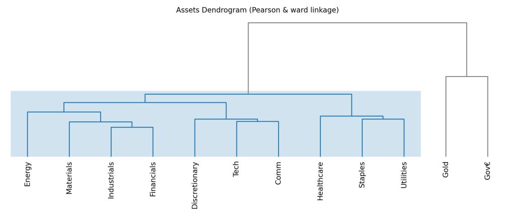
Let’s examine how the HERC algorithm performs with such a portfolio. Initially, HERC generates a dendrogram, as illustrated in Figure 8. Using this graphical representation, HERC automatically identifies sector indices and instruments with low correlation. Specifically, the 10 sector indices are grouped together, while gold and government bonds are placed on separate branches. This is a key advantage of hierarchical clustering, which organizes the portfolio without being swayed by the number of instruments within a particular asset class, such as equities.
HERC leverages the hierarchical structure to its advantage and, using the algorithm discussed in the previous section, allocates capital to balance risk equally across the tree’s nodes.
Figure 9 illustrates how the weights of the various portfolio components evolved between January 2020 and November 2023. This nearly four-year period was undeniably turbulent, marked by events such as pandemics, armed conflicts, and inflationary fluctuations, all of which significantly impacted financial markets.
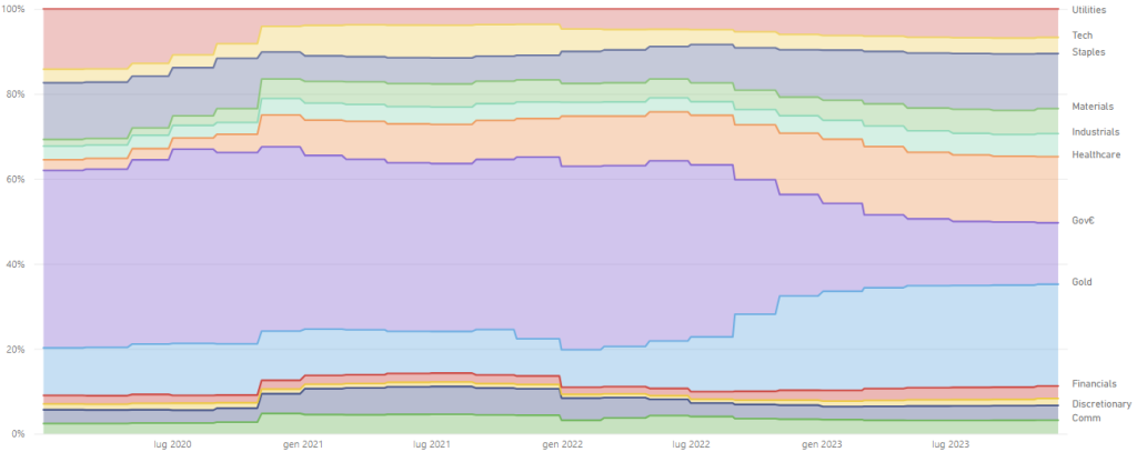
At the beginning of this period, government bonds accounted for approximately 40% of the entire portfolio – a significant proportion that gave our portfolio a profile resembling a classic “lazy” 60-40 allocation. During 2020, minor adjustments occurred, notably a reduction in the weight of the Utilities and Consumer Staples sectors, while the portfolio maintained stability and navigated periods of high volatility without overreacting.
However, starting in January 2022, with the first signs of inflation and the subsequent decline in bond values, a significant shift emerged. Gradually, the 40% share allocated to bonds dropped below 20%, making room for more defensive components like gold and consumer staples.
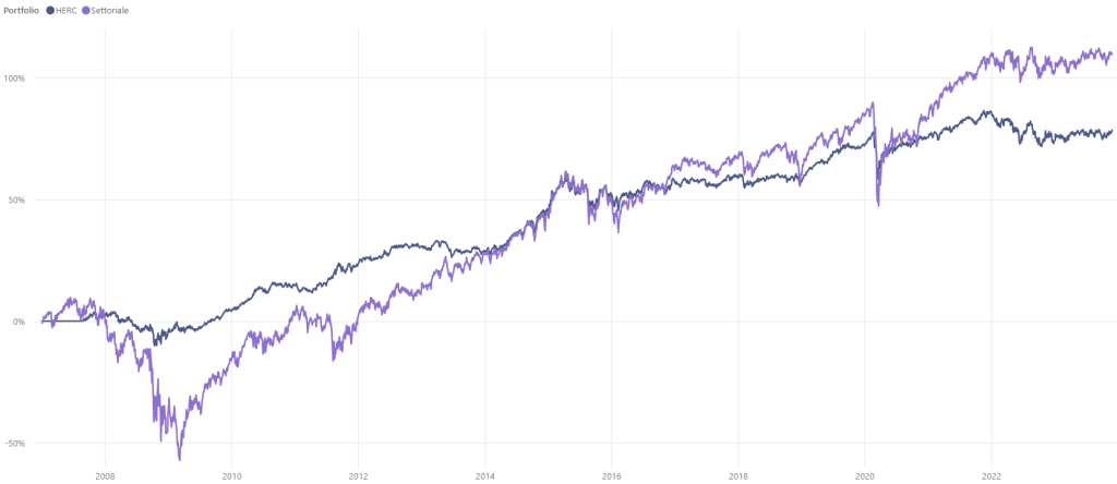
Figure 10 compares the performance curve of an exclusively equity-based investment with one that includes hedging. Even at a glance, it is evident that the hedged strategy offers greater stability. This becomes even more apparent when analyzing the drawdown, as shown in Figure 11, where the peaks are significantly reduced: the maximum drawdown decreases from approximately 50% to 18%. Additionally, recovery times are notably shorter with this strategy.
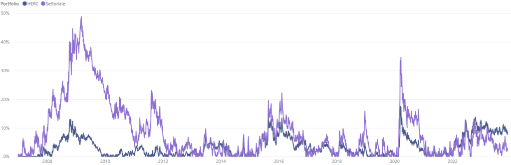
This is just one example of how a machine-learning-based model like HERC can autonomously make decisions to manage risk. HERC adjusts the allocation of capital among the portfolio’s various components to adapt to changing market conditions, showcasing its ability to dynamically adapt and manage risk effectively.
Conclusions and Future Perspectives
Markets are increasingly shaped by rapid and unpredictable dynamics, large-scale interventions by central banks, and global phenomena like wars and pandemics that influence investment decisions. These factors affect both small investors and large financial institutions. Today more than ever, risk management is crucial, often taking precedence over returns.
From my perspective, the Risk Parity approach provides a strong response to the challenges of a constantly evolving financial landscape. Hierarchical Equal Risk Contribution (HERC) is an intriguing evolution of this strategy, combining the principles of Risk Parity with Hierarchical Clustering to create a powerful methodology for constructing diversified and balanced portfolios.
However, it is essential to recognize that HERC is not a one-size-fits-all solution. Its strength is most evident when dealing with portfolios skewed toward a specific asset class, as demonstrated in our earlier example of a portfolio heavily weighted toward equities. Conversely, it is less effective in portfolios that are already well-diversified.
Implementing HERC is not a straightforward task, it requires more advanced computational tools than a typical Excel spreadsheet, such as Python and its specialized libraries for data science. This complexity, however, is the key to gaining a competitive edge and staying ahead in an ever-changing financial environment.
I would like to thank all the readers who have taken the time to reach the end of this article. I hope to have sparked curiosity about these fascinating methodologies and, above all, to have provided an accessible overview of a rarely discussed topic.
For those interested in exploring the HERC algorithm further, I recommend reading Thomas Raffinot’s original article, The Hierarchical Equal Risk Contribution Portfolio, which is available for free on the Social Science Research Network (SSRN). Additionally, I suggest an excellent article published on the website of Hudson & Thames, a FinTech company active in experimenting with new methodologies: Beyond Risk Parity the Hierarchical Equal Risk Contribution Algorithm.
In the next article, we will conclude the trilogy on hierarchical clustering by introducing the Hierarchical Risk Parity (HRP) algorithm, arguably the most significant and promising member of the Risk Parity family.
Happy investing!
If you have any questions to ask me, do not hesitate to write to me in the form below, otherwise you can find me on Facebook and LinkedIn. If you want to stay up-to-date and not miss any article as soon as it comes out, subscribe to the newsletter by filling out the following form:
If you like my articles and MP Investit project, you can support me with a free donation with PayPal. This encourage me to produce better and better content. Thank you!