

One of the rituals that we are used to doing on a regular basis is shopping at the supermarket. There are those who go in the evening on a midweek day, those who prefer Saturdays, others only when necessary. At my house my wife takes care of organizing it, from defining the list, checking offers, choosing the supermarket, selecting products on the shelf, paying at the cashier and arranging purchases in the pantry of the house. After all, women are extraordinary Program Managers, able to manage the entire cycle of an activity, without neglecting anything! When I am in the supermarket with her, I am not ashamed to say that my duty is simply pushing the cart! But this leaves me time to look around for something that can capture my attention and curiosity. There is one in particular that fascinates me, the convex mirror, like the ones in figure 1.

An unusual and sometime mysterious object, which has the ability to deform images and convey a very large space towards the observer compared to what a flat mirror would be able to do. After all, it has a practical functionality, it allows you to broaden the field of vision and, if installed in a shop, to easily control and manage thefts or unexpected situations.
The use of convex mirrors is extensive, on the streets we find them as traffic signs to visualize blind corners, or they are often used as objects of furniture. Even the art world was fascinated by it, personally my thoughts go to the painting “The Conversion of the Magdalene” by Caravaggio, where the Master uses a convex mirror to show the public the entry point of the light that illuminates Marta and Maddalena, making the light itself the real protagonist of the scene.

This digression brings us to the topic of this article, bonds. Anyone who has already read my articles is used to my practice to connect experiences of everyday life to the financial world, carried by the mathematical and engineering disciplines that are my own. Don’t be surprised that I’m able to find commonalities between a mirror and a credit note! The formula that determines the price of a bond has a shape that mathematicians call convex: just as a convex mirror can increase the field of view, a bond is able to amplify the effects of its variables on price changes.
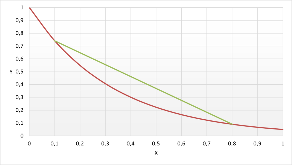
A graphical tool for the convex functions is shown in figure 3. With a red line we see a curve that splits the plane into two parts, a lower part and an upper one. If we take two random points of the curve and we join them with a straight line, the segment we obtain will always be in the upper half plane.
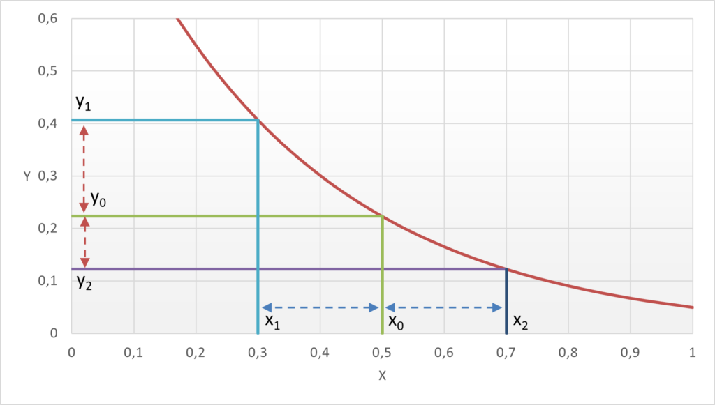
So far there is nothing exceptional about convex functions, but figure 4 introduces a feature that especially affects bonds. First, we choose a point x0 and, by moving first vertically and then horizontally (green line), we find the value y0 of the convex function. If now we take two other values x1 and x2 equidistant from x0, and we find the related values y1 and y2, we can see that the distance of y1 from y0 is significantly greater than the distance between y2 and y0. This feature can be explained as a distortion: two same variations of x, but in different directions, lead to different distances on the y axis.
The time has come to show which is the convex function that rules the price of a bond and how the distortion effect sets its behavior.
The price of a bond
Perhaps the main advantage of a bond as an investment tool is that its future is clear: unless extreme events such as issuer default or debt restructuring, a bond allows you to plan clearly and correctly the investment. This is not a negligible detail, think of two people who choose to invest the same amount of money, in the same company and at the same time, the first chooses to purchase a bond issued by this company while the second selects to buy shares. The investor who took the bond knows the cash flows and the value at maturity, the other one instead takes a leap in the dark, the dividends are settle from time to time and the value of the shares is fixed by the market.
We define a model that will have the following simplifying assumptions:
- The repaid maturity value is equal to its face value;
- The coupon is fixed and issued annually;
- The bond is in Euro and it does not depend on foreign currencies (no exchange rate risk);
- The face value of the bond is € 1000;
- The bond maturity date is set, without prepayments or default;
These hypotheses do not affect the quality of the model but they help to understand the model. Let’s see the formula for the price of bonds with all its grace, then let’s analyze and interpret it:
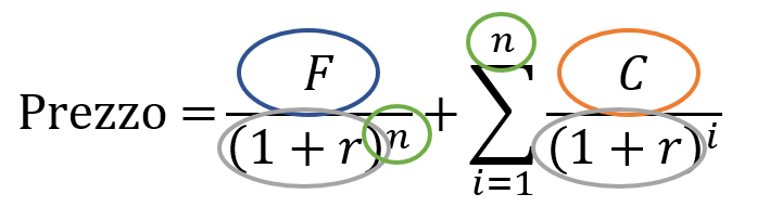
The colored ovals help us to identify its 4 variables:
- The face value F of the bond very often is the same of maturity price of the bond, therefore in the formula we find it in direct relationship with the price.
- The coupon value C proportionally affects the price, higher is its value and higher is bond price. The presence of the summation should not scare us, it reminds us that all coupons from now up to expiry must be added together to fix the price.
- At the denominator we find perhaps the most attractive term, the return r that the market expects to have on our bond.
- The number n of the years at the maturity of the bond has a double meaning, at the denominator it modifies the effects of the expected return r while in the summation it set the total flow of coupons to maturity.
A more in deep observation of these terms help us to note some important features of the formula:
- The face value F and the coupon value C are endogenous terms, meaning they are on inner side of the bond and someway they represent its structure, they are both in the numerator and therefore the higher their value, the higher the price of the bond. Under our assumptions, their values are fixed and they are set by the issuer at the issue of the bond.
- The expected return r is the exogenous term of the bond, meaning that it is on the external side and that there is no way to control it. The issuer’s degree of solvency, interest rates of the central banks, the market’s expectation of our bond, etc… all of them are inserted into the variable r. Its presence in the denominator has an inverse effect on the price, to have a high return, the price must necessarily be low.
As investors, we can know at any time in the life of the bond its face value F and its coupon C, but we can only speculate about the expected return r.
The summation is an important mathematical operator but it is not so flexible for an everyday use, to who wants to handle an easiest and more useful formula, I provide the following:
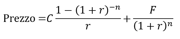
Compared to the first one, this formula has less intuitive terms to read into and, do not forget, the first term becomes null in the case of r = 0%.
Price changes over time
I think most of us, as investors, have seen and know the difference in volatility that a short-term bond can have compared to a long-term one. Bonds with little time to go are resilient to changes in the expected return and their price tends to remain stable, while bonds that still have a long way are subject to very large price variations.
Our formula can help us to visualize and better understand this behavior. Let’s take the case of a 2% fixed coupon and then we create a graph, where on the x-axis we find the years to maturity and on the vertical axis the price of the bond, while the coloured lines differ in the expected return.
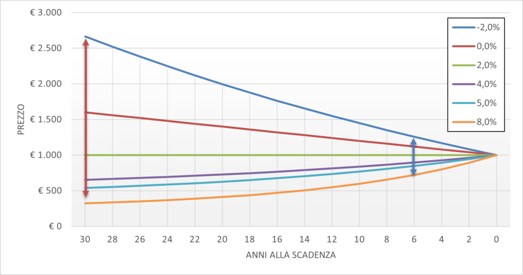
Let’s get started right away by noting how the highest expected returns of our coupon are always below the threshold of 1000€, our maturity price, while in the case of returns below 2% the price is always higher than the maturity price. The explanation is after all intuitive, if our bond provides a coupon lower than what the market expects, the price is lower than the maturity price to allow investors to have an additional profit.
The second matter to note is that the time remaining to maturity of the bond has the effect of modulating the effects of the expected return r. Bonds that have a maturity still far away have a very sensitive price from the expected return, in our example a residual maturity of 30 years leads to an incredibly high price spread (red vertical line), above 2300€. If the time to expiration is short, then this price variation is considerably reduced, in the case of 6 years remaining the window is about 500€.
The convexity of the formula is slightly hinted at, the price lines remain spaced apart for a long time and only in last years they curve more conviction to converge at the same point. A curiosity that a keen eye can notice is that the price lines that have a high expected return (those in the lower part of the graph) have a horizontal trend for most of the time, changing their slope only close to the maturity, while those with a low yield (the lines at the top of the graph) have the opposite effect, with a steep slope for long maturities that softens at shorter maturities. This is an important feature to know, if a bond is trading below its face value (1000€ in our example), the effect of the time is felt especially when there are few years to maturity, while if the bond is above the nominal value, time has a marked influence for the entire time frame.
Price changes over return
So far I hope that it is clear how the price changes over time, but we know well that the expected return (unfortunately) is never constant and it tends to change a lot over the years, under the dependence of so many variables which we partially listed above.
In Figure 6 we find the price formula for bonds from another point of view, as the expected return changes and for different values of years to maturity. We can admire the convexity of our formula, for instance the 30-years maturity starts from the top of the chart, then it quickly climbs down towards lower prices, it crosses the face value of 1000€ at the point where the expected return corresponds with the yield of the coupon, and then it flattens to the bottom. If the time distance from the maturity of the bond is reduced, the effect of convexity is less and the distance from the value of 1000€ is reduced.
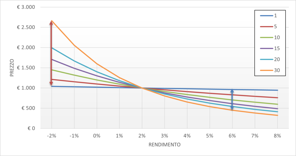
As in the previous figure, the price sensitivity from the expected return is very high for long maturities, while it is just appreciable at for short maturities. Let’s see a couple of examples to better understand what these curves want to tell us.
Decreasing yields
In the 2010s, we saw a continuous reduction of interest rates, which pushed some European government bonds to values well below zero. I remember when they touched 0% as yield, many people wondered if it made sense to hold similar bonds in the portfolio, especially if the trend was expected to have further decreases in yield. Let’s try to leave the bias out of such assessments and let’s ask the numbers what they think.
In Figure 7, an arrow has been inserted and it shows the price change of a bond with a 20-year maturity, in the event that the expected return falls from 0% to -1%. The price goes from 1400€ to 1668€, with a change of 19%! This is an incredible result for bonds, especially for those that have a very high credit rating like AAA! Bonds that start at much higher yields also get interesting results, for example the red arrow shows the variation from 6% to 5%, with a price gain of 16%.
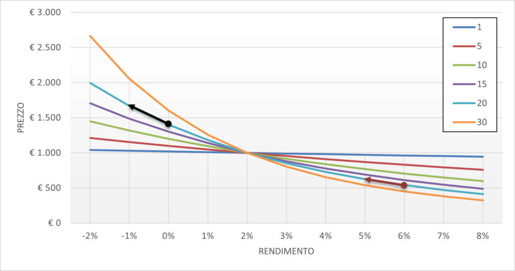
This observation leads us to the conclusion that if a generalized decline in expected yields is foreseen, it is more convenient to hold high-rated, high-maturity government bonds in the portfolio rather than high-yield bonds with little residual maturity.
Rising yields
Seen with some fear, rising interest rates are a recurring thought in the minds of investors. This reminds me of the famous quote “Winter is Coming” from “Game of Thrones”, where the House Stark of the North doesn’t stop getting ready for the arrival of an exceptional winter that would bring with it the threat of an unknown enemy.
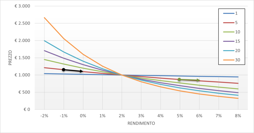
If long maturities were the favorites in the event of a drop in yields, now they become the most penalized ones, with a reduction of the same amount. Instead, if we observe a shorter maturity like the 5-years, an increase of 1% brings to 5% reduction for high-rated bonds (black arrow) and 4% for “High Yield” (green arrow).
Intuition suggests that we rely on safe government bonds in these market scenarios, but once again the numbers prove we’re wrong: convexity does not put bonds on the same level, but it favors those that already start from higher yield. To preserve capital in this market phase, it is suggested to have bonds with a low rating in the portfolio, such as “High Yield” Corporate, and especially with a low residual life, rather than government bonds issued by virtuous nations.
Case Study
The convexity of bonds is also valid for investment in bond funds such as ETFs. A fund consists of a basket of bonds and every bond differs from each others by coupon, maturity and provider, therefore it is not convenient to write a formula that include all these variables. Statistics can help us, it is always possible to take a picture of the basket and calculate the average values of coupons and maturities, even if they will not remain fixed over time. While estimating the behavior of a bond ETF is a winding road from a quantitative point of view, from a qualitative point of view it is feasible and the guidelines identified in this article always remain valid.
In this example we see two ETFs, the first with German Government Bonds as underlying index, ticker SDEU, the second with “High Yield” corporate bonds, ticker IHYG, both with iShares as provider. First, figure 9 shows the price changes in the last year of these two ETFs. If I asked you which of the two curves is the German Bund and which is the High Yield, I think in the heat of the moment most of us would answer that the Bund is the blue line and the red line is the High Yield. It is surprising to note that instead SDEU is the red line, with a much higher volatility, appreciable even with the naked eye, while IHYG had a more regular trend and only in the last period it followed the much more “risky” Bund!
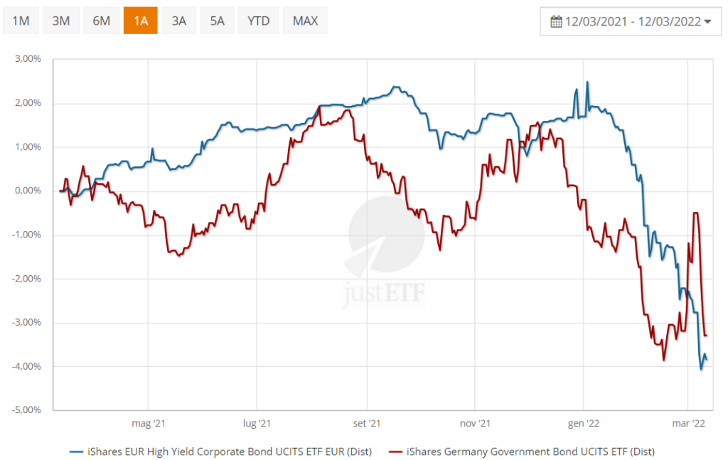
Is this a mistake or a trick? Neither, let’s try to draw the price curves with expected return as indipendent variable. At the time of writing, the data of these 2 ETFs are shown in the table below.
| SDEU | IHYG | |
| Face value | 1.000€ | 1.000€ |
| Weighted average coupon | 1,19% | 3,50% |
| Coupon frequency per year | 1 | 1 |
| Weighted average maturity | 9,14 | 3,99 |
| Expected return | -0,01% | 5,25% |
| PRICE | 1.110€ | 938€ |
Now we insert these data into the price formula and we draw the two curves (figure 10).
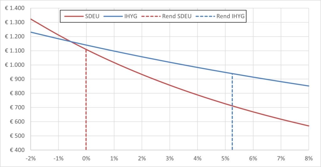
The vertical lines show the position of the expected return for the two ETFs, while the intersection with the price curve identifies the actual value of these two ETFs. The SDEU curve has a very steep slope around its current yield, which means that small changes in expected yield lead to much larger price changes. IHYG, on the other hand, is in a position where its curve has a flatter trend, therefore its prices have a lower sensitivity to the expected return.
Conclusions
After all this talk of price changes, variations in expected return and years to maturity, what we have learned is that we need to insert the right bond in the portfolio at the right time, possibly managing it when the situation turns in financial markets.
But there is a certainty that only bonds can give, that at maturity the price refund corresponds to its face value. Unless the issuer defaults, whoever buys a bond and chooses to bring it to maturity, can and must ignore the price changes, focusing only on the periodic distribution of the coupon.
Faites vos jeux!
Thanks
With the opportunity to looking for material on convex mirrors, this article was a good opportunity to discover Professor Emanuela Pulvirenti ‘s Didatticarte blog. I thank her its beautiful article convex mirrors and reflects of art which explores the convexity and its implication in the world of art.
For this article I have to thank Tyler, a mechanical engineer with a solid background in mathematics, a deep personal interest in finance and investment, and a great skill with Excel. Among the thousands of finance websites around the world, his Portfolio Charts is the one that really thrilled me, with his own narrative style, the ability to see things from original point of view, his sensitivity to look at the data as an engineer and the ability to communicate complex ideas to all people.
I came up with this article after I wrote an email to Tyler about his article on the convexity of bonds, and his subsequent answer in which he requested me to write and publish my own idea on this subject. I highly recommend reading his article:
At the end, I thanks who had the patience to read me so far and Happy Investing!
If you have any questions to ask me, do not hesitate to write to me in the form below, otherwise you can find me on Facebook and LinkedIn. If you want to stay up-to-date and not miss any article as soon as it comes out, subscribe to the newsletter by filling out the following form:
If you like my articles and MP Investit project, you can support me with a free donation with PayPal or with a Brave browser reward. This encourage me to produce better and better content. Thank you!