Predicting the Drawdown – a Machine Learning Model to Measure Risk (Part 4)

In this blog, I publish an article I wrote to take part in “SIAT Technical Analyst of the Year 2021” competition. Due to the length and quantity of the topics covered, I thought useful to split it into four parts. In this fourth part, we are going to use our model to predict the maximum drawdown and to draw conclusions.

Training, Validation and Testing

Once we have completed the data collection, the preparation part and the choice of the Machine Learning algorithm, the following step concerns the creation of the predictive model. A typical issue of Machine Learning is to run into an overfitting. It is a well-known problem of quantitative analysts that requires a validation process, such as with Out-of-Sample and In-Sample, or with Walk Forward Analysis methods.

For Machine Learning models, the process is split into two main phases:

• The available dataset consists of two parts, one is used to train the Machine Learning algorithm, which returns the predictive model, the other is used to evaluate the performance of the model;
• If the model passes the evaluation, it is trained again on the entire dataset and its predictions are tested with a new dataset.

In the same way as with trading systems, to use the same dataset for both training and validation of the model is a mistake, because if the model falls into an overfitting then it has memorized the entire dataset and the predictions of the same dataset will be with no doubt perfect, but if the model encounters new data that it has never seen before, it will not be able to predict. A common practice during the training phase is to use a cross-validation: the dataset is split into k smaller datasets, called folds or partitions; as many k models are trained, each of them on k-1 folders and then validated on the remaining folder; the prediction performances of the k models are compared with each other. Figure 12 shows the scheme of the two validation and testing phases applied to our project. The synthetic time series dataset is divided into three folders, three models are trained by crossing the two folders used for training and the one for validation. Each of the three models is trained on its own dataset and then predictive capabilities are test over data that it has not seen yet. This method can be computationally expensive, but it is an good solution for checking model performance and taking advantage of the available data.

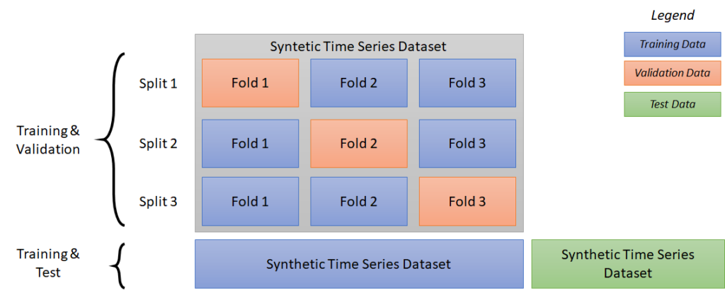
Once the validation phase has successfully passed and no overfitting issue has risen, the final model is created. As shown in Figure 12, the entire dataset of synthetic data is used again for training, without folders in order to maximize the yield of available data. The model so obtained will be tested with the real time series dataset, which the model has never seen before. It may seem complex to implement, but SciKit Learn handles everything implicitly with just two lines of code. For the details, you can consult the attached code.

Results

With the synthetic time series dataset and SciKit Learn‘s GridSearchCV function, validation results are obtained for three polynomial degrees, summarized in Table 5.

Polynomial Degree	Split 1 Score	Split 2 Score	Split 3 Score	Average Score
1	95.85%	95.59%	95.93%	95.79%
2	99.94%	99.94%	99.94%	99.94%
3	99.99%	99.99%	99.99%	99.99%

The score is calculate by the cost function and if it is close to unit it means that the algorithm is able to successfully create a predictive model. The third degree polynomial has the best performance, while the second degree is an excellent trade-off between performance and simplicity.

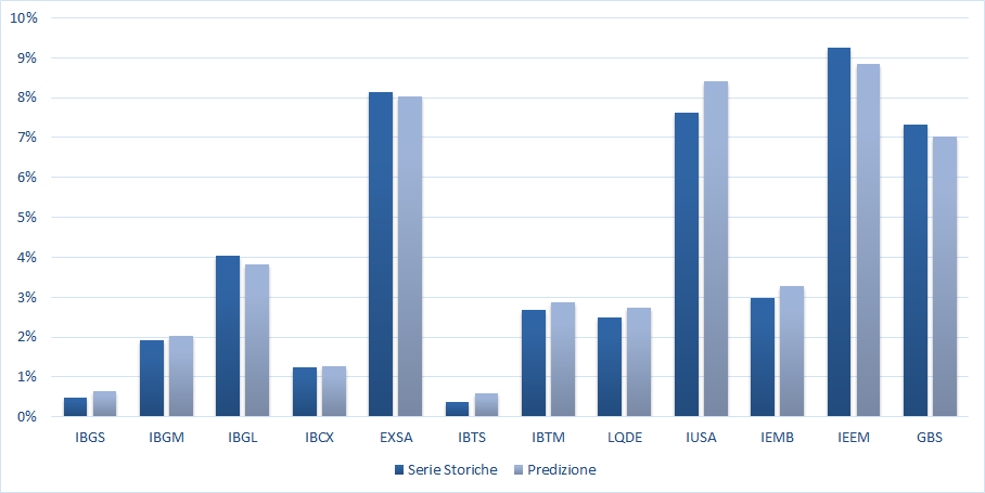
For the test phase, we choose the third polynomial degree and re-train the algorithm with all the synthetic time series dataset to maximize the yield of available data. Finally, the final model is created and, if fed with the dataset of real time series dataset (table 2), it provides predictions of the 90MDDs which, in figure 13, are compared with the real ones. The results are encouraging, the predictions are reliable and usually with nominal errors of 0.2%.

Let’s see in more detail how the final model is structured and how it works, for clarity we will illustrate the model with the second degree polynomial. When supplying a dataset to the model, for example as the dataset in Table 2, each row is recalculated as follows:

z₁ = z_µ = ( µ_i – µ_m ) / S_µ = ( µ_i – 2.01 · 10^-4 ) / 8.92 · 10^-5

z₂ = z_σ = ( σ_i – σ_m ) / S_σ = ( σ_i – 7.78 · 10^-3 ) / 4.20 · 10^-3

z₃ = z_T = ( T_i – T_m ) / S_T = ( T_i – 19.6 ) / 6.94

In this way, our data is standardized and normalized. Next, the polynomial regression creates the additional characteristics:

z₄ = z_µ² ; z₅ =z_µz_σ ; z₆ = z_µz_T ;
z₇ = z_σ² ; z₈ = z_σz_T ; z₉ = z_T²

In the end, the formula for predicting 90MDD is:

ŷ(β, z) = β₀ + β₁z₁ + β₂z₂ + β₃ z₃ + β₄z₄ + β₅z₅ + β₆z₆ + β₇z₇ + β₈z₈ + β₉z₉

Where the coefficients (found during training) are:

β₀ = 5.351% ; β₁ = -0.099% ; β₂ = 2.867% ; β₃ = 1.086% ; β₄ = 0.004%
β₅ = -0.005% ; β₆ = -0.037% ; β₇ = -0.041% ; β₈ = 0.609% ; β₉ = -0.122%

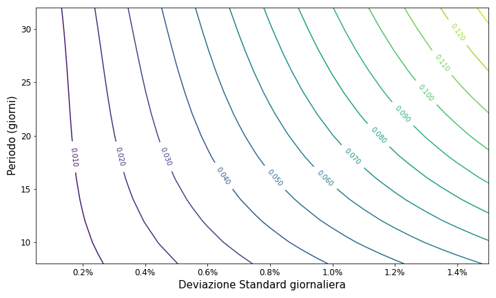
Figure 14 shows the weight of each individual coefficient in the prediction formula of 90MDD. Note how the main contribution comes from the intercept β₀, that is a constant value that is common to all predictions: we can state that each time series, regardless of the variables involved, will have a value of 90MDD that is always positive and far from zero. The second main contribution comes from the standard deviation, the greater its value the greater the 90MDD.

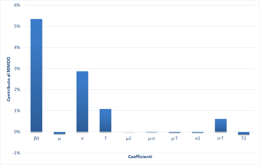
If we delete the terms with negligible coefficient value, we obtain a simplified formula that allows us to better highlight the main contributions to the 90MDD:

ŷ(z) = 5.351% – 0.099% · z_µ + 2.867% · z_σ + 1.086% · z_T + 0.609% · z_σz_T – 0.122% · z_T²

Previously in figure 5, we had already deduced the strong dependence of 90MDD from the standard deviation, and Machine Learning algorithm correctly used this dependence during the training phase. The average daily return has a negative contribution, while the period of the epochs contributes with its second degree terms too. The strong dependence that the MDD has from the standard deviation is a positive feature: the standard deviation usually is a robust statistical parameter, in the way that if we take some subsets of a time series and calculate the standard deviations, we will find results that are very close between them. This is not true for the return, it is less robust and it can change widely within a time series. To calculate the standard deviation over the entire time span of the time series or only over a subset is almost the same, as a consequence it allows us to always have reliable results.

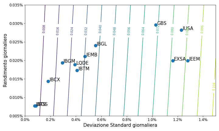
Figures 15 and 16 show a view of the formula ŷ(β, z) in the risk-return and risk-time plans, with the 90MDD isometric curves and with the dataset of real data for comparison (only in figure 15) . The verticality of the isometrics in the risk-return plan show how the dependence of 90MDD on the standard deviation is predominant with respect to the return, while in the risk-time plan, the period of the epochs has a greater influence on the right side of the graph, where the isometric curves are more skewed, indicating that the period contributes to 90MDD especially when it is amplified by the standard deviation.

Conclusions

“It is difficult to make predictions, especially about the future” this quote, attributed to the physicist Niels Bohr, encloses all the difficulties that exist in the Technical Analysis of the financial markets. The road that leads to predicting the future comes from the past: the main assumption is that there is a cyclic nature of the markets and that the events of the past can repeat themselves in the future, while backtests become the main tool for studying and analyzing strategies.

We have seen how generating a predictive model requires two main phases, the first is the definition of the rules that link the inputs with the outputs, the second is the execution of tests which, with the use of time series, allow to verify model capabilities to predict. In the traditional paradigm, the choice of rules is always a duty of the trader – programmer with his/her sensitivity and knowledge, while the machine takes care of testing them. With Machine Learning, on the other side, the choice of the rules of the predictive model is also delegated to the machine, leaving the human with a role of higher level as process supervisor.

What we have seen in this article is how it is possible to create a model that links the MDD with the expected return, the volatility and the observation period, leaving all the tasks to the machine, including validation and testing. What proposed relies on two important hypotheses:

• the distribution of returns must follow a “normal” one;
• mean and standard deviation of the distribution of returns are stable over time.

A normal distribution may be fine for non-derivative product such as indices and stocks, but to agree that an expected return is consistent over time reduces a lot the scope of our model. Furthermore, academia has already faced the problem of defining the distribution of MDDs, so why should we disturb the Machine Learning?

Machine Learning is very flexible, it has the capability to learn from provided dataset and to build a model on the data. The key to success depends on the quality and quantity of data, two properties guaranteed by synthetic time series:

• If we move our attention to the creation of more complex synthetic time series, then we will be able to have models that are not constrained by too pressing4 requirements. For example, it would be possible to define distributions for returns with some degrees of asymmetry, or to have a mean and standard deviation that change over time to simulate different market conditions, so that synthetic time series are closer to reality.
• The amount of information that can be created with a synthetic time series dataset is always enough for any statistical and Machine Learning analysis. In this article we have taken a relative short period of epochs, 20 days, but the user friendly high-level programming language and the high computing power of personal computers allow us to create thousands of time series over years-long intervals and to keep a timeframe as low as the daily one.

At the end, we remember how Machine Learning is able to lead qualitative analysis too: in the results paragraph we highlighted which are the variables that contribute most to the prediction, so Machine Learning allows us to feel the most inner side of the system and when there is knowledge, then there is also the awareness of how the world works.

Annex

Here below there is an extract of the code used to carry out the Machine Learning model.

Importing Libraries:

import numpy as np
import pandas as pd
import sqlite3 as sql
from sklearn.pipeline import Pipeline
from sklearn.model_selection import GridSearchCV
from sklearn.preprocessing import PolynomialFeatures
from sklearn.preprocessing import StandardScaler
from sklearn import linear_model

loading of the synthetic time series dataset, previously created and saved in a database:

conn = sql.connect('Synthetic.sqlite')
cur = conn.cursor()
DATASET = pd.read_sql('SELECT media, devst, periodo, MDD FROM dataset', conn)
conn.close()

Split of the dataset into one part with the input data and the other with the targets:

dataset = DATASET.iloc[:,:-1].to_numpy()
target  = DATASET.iloc[:, -1].to_numpy()

Model creation and validation:

Input = [('scale', StandardScaler()),
         ('polynomial', PolynomialFeatures(degree = 2, include_bias = False)),
         ('linearregression',linear_model.LinearRegression())]
Pipe1 = Pipeline(Input)
griglia = GridSearchCV( estimator = Pipe1,
                       param_grid = {'polynomial__degree' : [1, 2, 3]},
                       cv = 3)
griglia.fit(dataset, target)
pd.DataFrame(griglia.cv_results_)

Training with the whole dataset:

Input = [('scale', StandardScaler()),
         ('polynomial', PolynomialFeatures(degree = 3, include_bias = False)),
         ('linearregression',linear_model.LinearRegression())]
Pipe2 = Pipeline(Input)
Pipe2.fit(dataset, target)

Print of standardization parameters (mean and variance):

print('media', Pipe2[0].mean_)
print('varianza', Pipe2[0].var_)

Print of Linear Regressor attributes (intercept β₀ and coefficients β_x):

print('intercept', Pipe2[2].intercept_)
print('coefficient',Pipe2[2].coef_)

---

If you have any questions to ask me, do not hesitate to write to me in the form below, otherwise you can find me on Facebook and LinkedIn. If you want to stay up-to-date and not miss any article as soon as it comes out, subscribe to the newsletter by filling out the following form:

If you like my articles and MP Investit project, you can support me with a free donation with PayPal or with a Brave browser reward. This encourage me to produce better and better content. Thank you!