
Markowitz’s approach to building financial portfolios, known as Modern Portfolio Theory (MPT), revolutionized the financial world by introducing key concepts like diversification and portfolio optimization. Central to this theory is the mathematical model that quantifies the trade-off between risk and return.
In this article, we will tell his story and how he started from a simple yet revolutionary idea for his time to create a tool capable of finding efficient portfolios. We will not limit ourselves to describing the MPT model but will transform mathematical equations into geometric forms to provide a visual perspective that facilitates the understanding of a complex concept of the model, the Critical Line.
Challenging Authority
The protagonist of our article is Harry M. Markowitz, born in Chicago in 1927. It was a time marked by the Great Depression, but his parents, owners of a small grocery store, managed to live a respectable life, living in a nice apartment where young Harry had a room all to himself and provided him with support for his schooling.
From a young age, Harry showed an insatiable intellectual curiosity, attracted to various disciplines such as astronomy and philosophy, and also found pleasure in artistic expression through music and reading adventure stories. When he started attending the University of Chicago, Harry tried to maintain this variety of interests, but the academic path required the young student to specialize in more advanced courses. Harry thought it over and decided to dedicate himself to Economics.
Harry found himself immersed in a stimulating academic environment, alongside prominent professors who promoted economic research and were capable of influencing the country’s economic thought. He became particularly passionate about the “economics of uncertainty,” diving into theories on the utility function of Friedman and Savage, both his teachers at the university, and attending Koopmans’ course on efficient set analysis.

The turning point for Harry came when he considered the possible topic for his Doctoral Thesis. After a conversation with his professor Jacob Marschak, he decided to delve into the applications of econometric theories, intrigued by their application to stock markets. The first step was to compile a list of books that could guide him in exploring the state of the art in financial mathematics of the time.
Imagine the environment Harry Markowitz found himself in the early 1950s. In an era without the internet and search engines offering unlimited access to information, the primary source of learning was the library — stern and silent spaces where students spent hours reading articles and manuals. This approach to study was predominantly closed: texts were directly selected by professors and reflected formally accepted theories, following guidelines without questioning them. Moreover, students had few alternatives to interact with others besides the same university circle. There were no online forums or social groups connecting people from all over the world with different cultural backgrounds and unique study and professional paths.

In such a context, the main goal of students working on their Theses was to obtain professors’ approval. Consequently, few were inclined to deviate from common thinking and challenge conventional ideas, preferring the safer path to academic recognition.
Challenging convention is no ordinary act, especially in the most respected academic circles where authority is a big deal.
https://portfoliocharts.com/2023/07/10/remembering-harry-markowitz/
Except for one. Harry was an exception, endowed with an open mind and eager to think innovatively, he had developed from a young age a passion for a wide range of subjects, each of which contributed to shaping his way of seeing the world. This diversity of interests allowed him to explore different perspectives and points of view, never limiting himself to uncritically accepting the theories recommended by his professors. Let’s read Harry’s words directly:
The basic concepts of portfolio theory came to me one afternoon in the library while reading John Burr Williams’s Theory of Investment Value. Williams proposed that the value of a stock should equal the present value of its future dividends. Since future dividends are uncertain, I interpreted Williams’s proposal to be to value a stock by its expected future dividends. But if the investor were only interested in expected values of securities, he or she would only be interested in the expected value of the portfolio; and to maximize the expected value of a portfolio one need invest only in a single security. This, I knew, was not the way investors did or should act.
https://www.nobelprize.org/prizes/economic-sciences/1990/markowitz/biographical/
Williams’ approach was typically academic, reflecting an idea far removed from the real world. Harry, coming from a middle-class family, understood well that investors do not concentrate all their capital in a single asset due to risk aversion. The theories of his professors focused primarily on returns, neglecting the concept of risk. Harry’s revolutionary idea was to introduce risk as a new parameter alongside returns, in order to develop a new financial model capable of meeting the real needs of investors.
It was during this period that Harry took paper and pen, drew risk on one axis, returns on the other, and sketched a small figure that would later be called the “Efficient Frontier,” the first in history. The Portfolio Theory was being born.
After completing his PhD Thesis, the discussion was a success; the committee recognized the value and merit of his work, which centered on the human instinct to manage risk, even though it challenged the authority of the great minds of economics. It is said that during the discussion of his Thesis, Harry had to face a sharp remark from Professor Friedman: “We cannot award you a PhD in economics for a thesis that does not deal with economics.” Friedman was, of course, joking, and Harry earned his well-deserved degree.
The Efficient Portfolio Model
Harry Markowitz’s contribution did not stop at introducing a new financial paradigm known as Modern Portfolio Theory (MPT), but he also distinguished himself by defining this economic theory with mathematical rigor, a real revolution for the time.
In his article “Portfolio Selection” published in The Journal of Finance in 1952, Harry outlines the mathematical model that synthesizes his theory:
 \tag{1}
\begin{cases}
\min \limits_w \displaystyle \sum_{i,j=1}^N w_i w_j \sigma_i \sigma_j = V^* \\
\displaystyle \sum_{i=1}^N w_i E \lparen R_i \rparen = R^* \\
\displaystyle \sum_{i=1}^N w_i  = 1 \\
w_i \ge 0 \text{  } \lparen con \text{ }i=1, \dots ,N \rparen
\end{cases}
The summation in the first row allows calculating the portfolio’s variance, which depends on three variables: the weights (wi) of the assets within the portfolio; the standard deviation (σ) of each individual asset; and the correlation (ρ) between the assets. The standard deviations of the individual assets and the correlation are endogenous factors determined by the behavior of the financial assets in our hypothetical basket and are therefore not modifiable. The weights, on the other hand, are our design variables that we can manipulate at our discretion to determine the optimal portfolio composition.
The goal of this model is to identify the combination of weights (wi) that provides the minimum portfolio variance. However, the selection of weights is not free but must meet three fundamental constraints: the expected return of the portfolio must equal a predetermined value (R*); the weights must use the entire available capital; the weights must be positive, thus avoiding the opening of short positions.
In other words, the mathematical model asks us to find the weights (wi) of the financial assets that guarantee the lowest possible risk for a given expected return value. Easier said than done! The model requires finding a minimum value of a quadratic function, which is subject to linear constraints with both equalities and inequalities: a problem without a solution expressible as a combination of mathematical functions and valid globally. We are therefore in a stalemate situation because solving the problem is more complex than it seems.
The Critical Line
I admit that mathematical equations can appear cold and inflexible, but if we transform them into a geometric form, it becomes possible to more clearly understand the MPT model and the idea behind the theory. The following graphical representation is the same proposed by Markowitz himself in his works, considering a case study with three financial assets.
If we take up the set of equations and inequalities (1) and set N=3, the model simplifies as follows:
 \tag{2}
\begin{cases}
\min \limits_w V \lparen w_1 , w_2, w_3 \rparen =
\min \limits_w \lparen w_1^2 \sigma_1^2  + w_2^2 \sigma_2^2 + w_3^2 \sigma_3^2 + \\
+2w_1 w_2 \sigma_1 \sigma_2 \rho_{12}+2 w_1 w_3 \sigma_1 \sigma_3 \sigma_{13}+2 w_2 w_3 \sigma_2 \sigma_3 \rho_{23} \rparen = V^* \\

R \lparen w_1 , w_2, w_3 \rparen =
w_1 E \lparen R_1 \rparen + w_2 E \lparen R_2 \rparen + w_3 E \lparen R_3 \rparen = R^* \\

w_1 + w_2 + w_3  = 1 \\

w_1 ; w_2 ; w_3  \ge 0 \\

\end{cases}
The third equation can be rewritten as w3=1-w1-w2 and if we substitute into the other expressions, we obtain:
 \tag{3}
\begin{cases}
\min \limits_w V \lparen w_1 , w_2 \rparen = V^* \\
R \lparen w_1 , w_2 \rparen = R^* \\

w_1  \ge 0 \\
w_2 \ge 0 \\
1 - w_1 - w_2  \ge 0 \\
\end{cases}
The expected return and variance are thus expressed through two variables, as well as the three inequalities, which allow us to operate on a Cartesian plane and easily draw the equations and inequalities of our model.
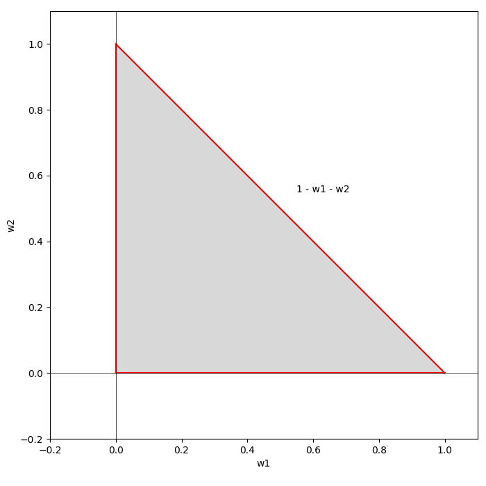
When represented on the Cartesian plane, the three inequalities transform into three lines that define a right isosceles triangle, as shown in figure 3. The area enclosed by the triangle includes all combinations of w1 and w2 that meet the constraints of our model (3). Any point outside the triangle violates the inequalities; for example, to the left of the triangle, we will have w1<0, while to the right, we will have 1-w1-w2>0.
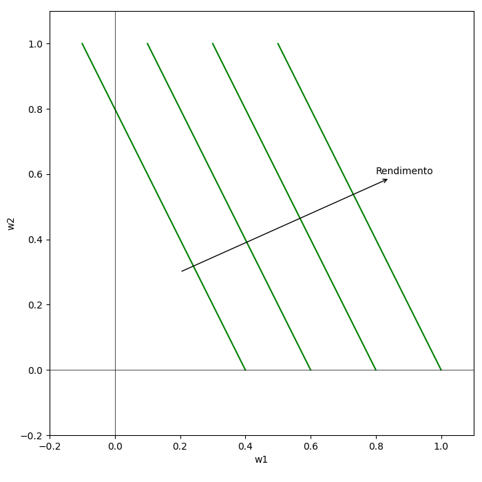
The second equation relates to the portfolio return, becoming a line in the Cartesian plane. As shown in figure 4, if we modify the target return R*, we obtain a series of parallel lines, where the lines further to the right have higher values of R*.
On the other hand, the first equation, which calculates the portfolio variance, has the characteristic of being quadratic. Graphically, this translates into a series of ellipses, whose dimensions vary with the target value V*. All these ellipses share a common center, which also coincides with the point where the variance is minimal.
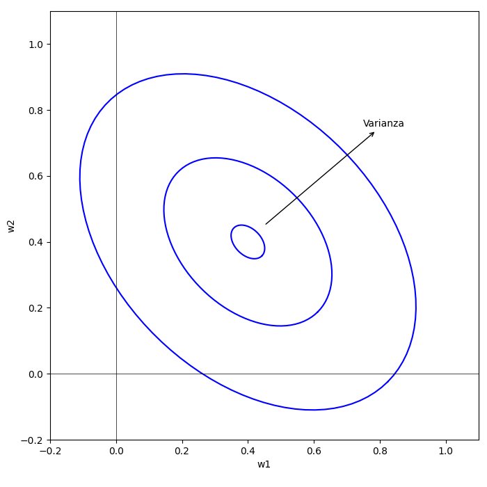
Now, our goal is to find the combination of weights w1 and w2 that lead to the minimum variance value. If we were to rely solely on the variance equation, it would be sufficient to take the coordinates of the ellipse’s center, and the problem would be solved. However, the presence of the four constraints requires us to identify the ellipse closest to its center that meets these constraints.
Graphically, if we overlay the three figures, the ellipse, to be a valid solution, must have a part within the triangle and must intersect the target return line R*. From the graph in figure 6, it is evident that the smallest ellipse is the one tangent to the line R* and corresponds to our solution V*.
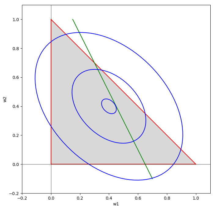
The intersection point in figure 6 satisfies all the expressions present in our mathematical model (3), as it is located within the triangle of inequalities and lies both on the target return line R* and on the variance ellipse V*. The coordinates of this point, identified by the weights w1 and w2, represent the solution to our problem.
Let’s now try to repeat the same exercise, but by taking a new target return line, for example, slightly shifted to the right. We will find a new point as the intersection between the target return line and the variance ellipse, slightly shifted to the right. By repeating this procedure for different values of R*, we will be able to draw a line that connects all our solutions, as illustrated in figure 7.
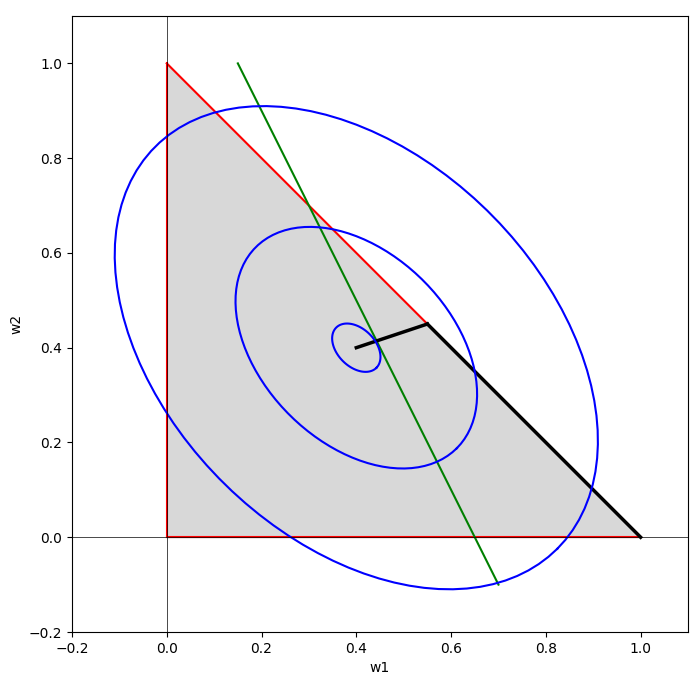
This line ideally starts from the center of the variance ellipses, moves to the right until it meets the hypotenuse of the triangle of inequalities, and then continues along it until it reaches one of the two vertices of the triangle.
This broken line is known as the “Critical Line,” as formulated by Harry Markowitz in his major works. The Critical Line allows for the determination of the set of efficient portfolios, i.e., all combinations of weights wi that minimize risk as the target return R* varies:
 \tag{4}
\lparen w_1 , w_2 \rparen = f_{CL} \lparen R^* \rparen
Finding a solution by intersecting only lines and segments is generally simple, but among our figures, we also have an ellipse, which, with its curved lines, increases the level of complexity to the point that we are unable to find an analytical solution. If we have a portfolio with only three instruments, as in our case, we are still able to draw the Critical Line, but if the number of instruments increases even by a few units, we will no longer be able to draw functions in multi-dimensional spaces, let alone find a Critical Line.
This is the real obstacle of the efficient portfolio model: the presence of a quadratic function makes it impossible to find a general formula for the Critical Line that is always valid for a generic set of assets.
A mathematical model without a solution is like a compass without a needle: useless and unable to guide in the desired direction.
But Harry had an ace up his sleeve.
Critical Line Algorithm
For centuries, mathematicians have encountered situations where elegant and refined mathematical models captured the essence of natural phenomena but lacked closed-form solutions to reveal their secrets. Although it is possible to apply assumptions to simplify the structure of models and thus arrive at solutions, these remain limited to particular cases, more useful for study purposes than for practical applications. The Markowitz model, which governs Modern Portfolio Theory, also finds itself in this situation, with closed-form solutions available only in special cases, such as portfolios composed of only two instruments or with zero correlations.
In the 19th century, a new approach emerged to tackle the problem of solving mathematical models: numerical analysis. This discipline, which falls under the broader category of applied mathematics, aims to solve mathematical models using the concept of approximation. The basic idea is quite simple: if there are clear limits in finding exact solutions, why not seek solutions similar to the original, differing by a relatively small error? Between 1800 and 1900, many numerical methods were developed, such as interpolation, least squares, and Monte Carlo methods, which paved the way for the widespread use of mathematics in a wide range of practical applications.
There is always a downside. Although numerical analysis offers undeniable advantages and can find solutions to a broad range of mathematical problems, its biggest drawback is the computational cost, such as sums or multiplications, which grow exponentially with the increase in the required precision. For decades, the computational cost was a real brake on the development of numerical analysis. After all, why engage in the study and definition of a numerical method if there is no way to perform the countless calculations required?
In the second half of the 20th century, numerical analysis underwent a revolution with the advent of the first computers equipped with efficient and innovative transistors, designed specifically to perform calculations at a speed impossible for any human being, with impeccable precision and at an acceptable economic cost. Computers quickly spread among research institutions, finally allowing the transition from theory to practice.
Harry Markowitz found himself in the ideal historical moment: the problem posed by his efficient portfolio model could have a solution. His intellectual curiosity and multidisciplinary approach were crucial in studying and mastering a subject as complex as numerical analysis.
In 1951, near the end of his academic studies, Harry met some individuals working at the RAND Corporation, a company specializing in research and development across various fields, including the creation of optimization and simulation methods to solve mathematical models used to analyze and resolve complex decision-making problems. The RAND Corporation had the exact knowledge Harry needed to solve his efficient portfolio model.
The RAND Corporation offered Harry a job, and he did not hesitate to move from Chicago to California. There, he found a highly stimulating work environment, composed of brilliant minds like George Dantzig, a mathematician specializing in applied mathematics and an expert in optimization processes. Dantzig was famous for having invented the simplex algorithm, used to solve linear programming problems, a type of mathematical model not very different from that of efficient portfolios.
Harry took advantage of this fertile environment and soon became an expert in numerical analysis, optimization techniques, and computer programming. He then began to study a specific algorithm for his Critical Line that could find a solution once expected returns, variances, and covariances were known, for any number of assets and subject to various types of constraints. The result of this work was called the Critical Line Algorithm (CLA) and was published in 1956. This algorithm was specifically designed for the optimization of portfolios subject to inequality constraints and ensures that a solution is found after a fixed number of iterations.
I will avoid explaining the mechanisms of this algorithm, as I don’t want to bore anyone with matrix notations and Lagrange multipliers. I’ll let Harry’s own words explain how the algorithm works and what the relationship is between the Critical Line and efficient portfolios:
“Imagine the Critical Line as railway tracks. Imagine, further, that a passenger boards a train at X and travels in the direction of increasing expected return. The first time his train crosses another track – as soon as the first critical line intersects a second critical line – the passenger transfers to the new track, the new critical line, and again travels in the direction of increasing expected returns. Again he reaches another track, an intersection of critical lines, and again he transfers to the new, continuing in the direction of increasing expected return. This continues until the passenger reaches X with maximum expected return. There his journey ends.”
Each point crossed by the passenger during his journey represents an efficient portfolio. In Figure 9, for example, the set of efficient portfolios is represented by the thicker line, which starts at point X, moves along the Critical Line L1,2,3,4, intersects the Critical Line L1,2,3, which in turn intersects L2,3, and reaches the final point X2.
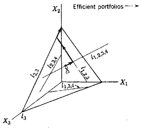
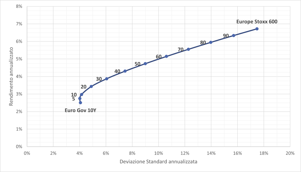
This path, which Harry plotted on a Cartesian coordinate system with the weights w1, w2 and w3 along the axes, when transposed onto a new Cartesian plane with variance on the horizontal axis and return on the vertical axis, leads us to a line familiar to many of us: the efficient frontier.
Between Success and Challenges
Harry Markowitz left an indelible mark on portfolio theory. His ideas and revolutionary approach quickly spread, not only in academic circles but also in the world of investments. Banks, fund managers, financial advisors, independent investors, and even enthusiasts: all are familiar with and have at least once constructed and utilized the efficient frontier for their own portfolios.
This extraordinary success has led to the widespread production of books, articles, and informational materials, which are now easily accessible on the internet. As often happens, those approaching the study of efficient portfolio theory typically do so through texts that reinterpret Markowitz’s original ideas, rather than through the original texts published in the 1950s. Although it’s not wrong to study from derivative texts, this can lead to the spread of misconceptions and an incorrect assessment of the theory’s strengths and weaknesses.
Let’s review some criticisms and preconceptions of the model proposed by Harry Markowitz:
- Parameter Estimation Based on Historical Data. It is often assumed that constructing the efficient frontier requires estimating expected returns and variances based on historical price series. However, Markowitz never claimed this to be the correct method for estimating parameters. He emphasized that parameter estimation is a separate topic and should not be conflated with the capital allocation problem. While using historical data is the simplest approach, it is certainly not the most accurate or reliable.
- Risk Measurement Through Variance. The model uses variance as a measure of risk, which assumes that the distribution of returns approximates a normal distribution. This assumption does not account for asymmetries and the shape of the tails in return distributions. Although this hypothesis is valid in many cases, it is not applicable in others, such as options or certificates. Moreover, variance does not differentiate between negative returns, which result in undesirable losses for investors, and positive returns, which are desirable.
- Lack of a Temporal Variable. The model does not consider the time factor, but from experience, we know that expected returns and correlations between asset classes can vary significantly depending on economic scenarios, as do investor risk and return expectations. Additionally, the weights of the assets within the portfolio are continuously changing, making it impossible to maintain the fixed allocations predicted by the model. While it is possible to perform new estimations and rebalancing at predetermined intervals, these are approximations that do not fully capture the behavior of a portfolio as market conditions change.
- Portfolio Diversification. Markowitz’s initial idea, which later led to his theory, was that a portfolio should be well diversified rather than concentrated in a few assets. However, the proposed model is not inherently capable of ensuring good diversification. Typically, portfolios on the efficient frontier are those that concentrate capital in a few assets, thereby undermining the benefit of diversification. Paradoxically, even if the basket size is increased, the model would still focus on a few assets, not benefiting from the presence of more securities.
A diversified portfolio means having a higher chance that the portfolio will generate returns in line with expectations, reducing the specific risk that one or more assets could generate losses. In contrast, with a poorly diversified portfolio, such as those on the efficient frontier, the performance heavily relies on the outcomes of a few assets. - Instability. If we slightly modify the values of our parameters, the model is considered stable if the final solution also changes by a small percentage. Unfortunately, Markowitz’s model does not exhibit good stability, particularly concerning returns. This means that if expected returns are not estimated with enough accuracy, the efficient frontier obtained will differ significantly from the one generated by future data.
Many decades later, the theory advanced by Harry Markowitz remains the primary reference point for both small and large investors. This model has significantly influenced – and continues to influence – all modern portfolio construction theories. Why, despite the limitations and flaws previously mentioned, has this model been so successful and why does it continue to thrive today?
We often take for granted the difficulties faced by pioneers. In the 1950s, concepts like diversification and risk management were practically nonexistent. Moreover, the near-total absence of computers meant that calculations were carried out manually by legions of “human calculators.” In this context, Harry Markowitz had the merit of introducing the concepts of diversification and risk into portfolio theory with the scientific rigor typical of the experimental method, involving observation, hypothesis, and experimentation. He developed a model that encapsulated all these concepts, making intensive use of the emerging computing technology.
These achievements cannot be underestimated or considered secondary. Markowitz’s ability to integrate theory and practice, to foresee the importance of risk management, and to leverage emerging technologies to solve complex problems, explains the enduring success of his theory. For me, this is the reason behind the lasting success of Harry Markowitz.
Further Reading
Even though it’s a challenging read, Harry Markowitz’s 1959 book, “Portfolio Selection: Efficient Diversification of Investments”, is the foundational text that compiles all his work on efficient portfolio theory. In this volume, Markowitz provides a detailed definition of his model and explores the mathematics behind it, offering a comprehensive discussion of the Critical Line.
To fully grasp the impact of the computer revolution in the scientific and engineering fields, I highly recommend watching the movie “Hidden Figures”. This film tells the story of Katherine Johnson, an African American mathematician who worked as a “human computer,” performing manual calculations crucial for data processing. The arrival of the IBM 7090, one of the first transistorized computers, which Markowitz also used, exponentially increased computational capabilities but challenged the role of human calculators. The film’s protagonist, along with her two best friends and colleagues, had to adapt to the changing times, return to study, and seize the opportunities offered by the new emerging professions within NASA. The film also highlights how these women overcame harsh racial discrimination, serving as examples of resilience and adaptation during an era of technological and social change.
Happy investing!
If you have any questions to ask me, do not hesitate to write to me in the form below, otherwise you can find me on Facebook and LinkedIn. If you want to stay up-to-date and not miss any article as soon as it comes out, subscribe to the newsletter by filling out the following form:
If you like my articles and MP Investit project, you can support me with a free donation with PayPal. This encourage me to produce better and better content. Thank you!